
Cambridge 2025
Checkout using your account
Este formulario está protegido por reCAPTCHA: se aplican la Política de privacidad y las Condiciones del servicio de Google.
Checkout as a new customer
Creating an account has many benefits:
Rápido. Preciso. Fácil de usar. Stata es un paquete de software completo e integrado que cubre todas sus necesidades de ciencia de datos: manipulación de datos, visualización, estadísticas e informes automatizados.
Novedades de Stata 19
Comprar Stata para empresas, gobiernos, organizaciones sin fines de lucro, instituciones educativas o estudiantes.
| OS | Windows 10 Macs with Apple Silicon and macOS 10.13 or newer for Macs with Intel processors |
|---|---|
| Processor | Applie Silicon, Intel or AMD processor (Core i3 equivalent or better) |
| Memory | Stata/MP > 4GB, Stata/SE > 2GB, and Stata/BE 1GB |
| Hard Drive | 4GB |
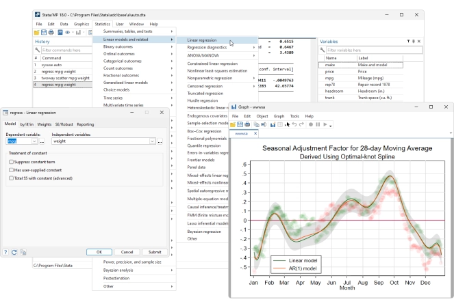
Data Management
Statistics
Graphics
Rápido. Preciso. Fácil de usar. Stata es un paquete de software completo e integrado que cubre todas sus necesidades de ciencia de datos: manipulación de datos, visualización, estadísticas e informes automatizados.
|
|
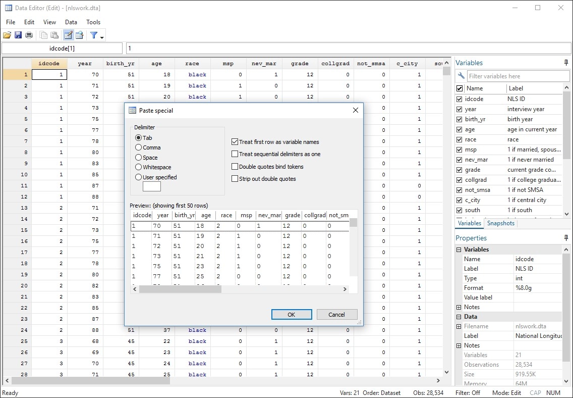
Las funciones de gestión de datos de Stata le brindan control total.
|
|
Stata facilita la generación de gráficos con un estilo distintivo y con calidad de publicación.
Puedes apuntar y hacer clic para crear un gráfico personalizado. O puedes escribir scripts para producir cientos o miles de gráficos de forma reproducible.
Exporte gráficos a EPS o TIFF para publicación, a PNG o SVG para la web, o a PDF para visualización.
Con el Editor de gráficos integrado, puede hacer clic para cambiar cualquier aspecto de su gráfico o para agregar títulos, notas, líneas, flechas y texto.
Todas las herramientas que necesitas para automatizar el informe de tus resultados.
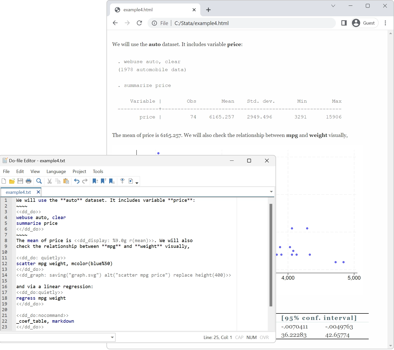
Mucha gente habla de investigación reproducible. Stata se ha dedicado a ello durante más de 40 años.
Constantemente añadimos nuevas funciones; incluso hemos modificado radicalmente elementos del lenguaje. No importa. Stata es el único paquete estadístico con control de versiones integrado. Si escribiste un script para realizar un análisis en 1985, ese mismo script seguirá ejecutándose y produciendo los mismos resultados hoy. Cualquier conjunto de datos que creaste en 1985, podrás leerlo hoy. Y lo mismo ocurrirá en 2050. Stata podrá ejecutar cualquier cosa que hagas hoy.
Nos tomamos muy en serio la reproducibilidad.
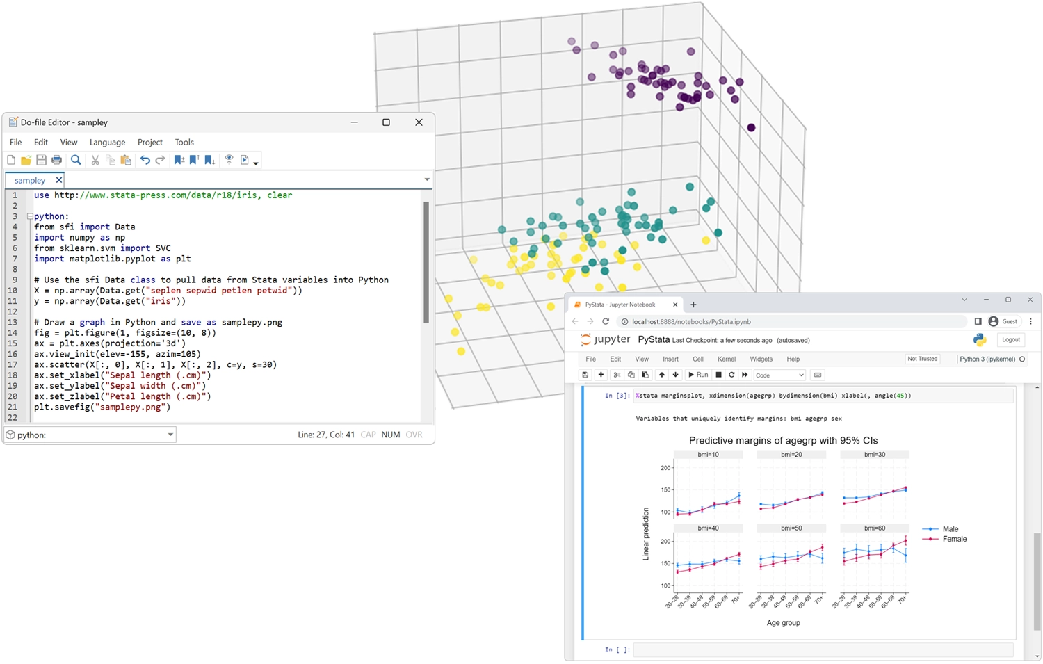
Invoque Python de forma interactiva o incorpore Python en su código Stata.
Invocar Stata desde Python y llamar al código Stata desde entornos IPython.
Utilice Stata dentro de Jupyter Notebook.
Transfiera datos y resultados sin problemas entre Stata y Python.
Utilice los análisis de Stata desde Python.
Utilice cualquier paquete de Python dentro de Stata
Cuando llega el momento de realizar sus análisis o comprender los métodos que está utilizando, Stata no lo deja abandonado a su suerte ni lo obliga a pedir libros para aprender cada detalle.
Cada una de nuestras funciones de gestión de datos está completamente explicada y documentada, y se muestra en la práctica con ejemplos reales. Cada estimador está completamente documentado e incluye varios ejemplos con datos reales, con explicaciones reales sobre cómo interpretar los resultados. Los ejemplos le proporcionan los datos para que pueda trabajar con Stata e incluso ampliar los análisis. Le ofrecemos una guía de inicio rápido para cada función, mostrando algunos de los usos más comunes. ¿Desea obtener más detalles? Nuestras secciones de Métodos y fórmulas proporcionan los detalles de lo que se calcula, y nuestras Referencias le indican aún más información.
Stata es un paquete grande y, por lo tanto, cuenta con mucha documentación: más de 19 000 páginas en 36 manuales. Pero no te preocupes, escribe "ayuda con mi tema" y Stata buscará en sus palabras clave, índices e incluso en paquetes aportados por la comunidad para ofrecerte toda la información que necesitas sobre tu tema. Todo está disponible directamente en Stata.
No solo programamos métodos estadísticos, los validamos.
Los resultados que obtiene de un estimador de Stata se basan en comparaciones con otros estimadores, simulaciones de Monte Carlo de consistencia y cobertura, y exhaustivas pruebas realizadas por nuestros estadísticos. Todos los productos de Stata que entregamos han superado un paquete de certificación que incluye 7,2 millones de líneas de código de prueba que generan 6 millones de líneas de salida. Certificamos cada número y fragmento de texto de esos 5,8 millones de líneas de salida.
Durante más de 40 años, StataCorp ha sido fiel a sus usuarios, expandiendo el software Stata con nuevos métodos estadísticos y lo último en generación de informes, visualización y manipulación de datos, así como en la interfaz de usuario. Gracias a nuestra larga trayectoria de lanzamientos, nos comprometemos a proporcionar continuamente un software estable y confiable a nuestra diversa comunidad de investigadores y profesionales.
![]()
Mantenerse actualizado con la versión más actualizada de Stata ahora es más fácil que nunca.
StataCorp desarrolla continuamente nuevas funciones para mejorar el software Stata, desde los métodos estadísticos más recientes hasta la mejor generación de informes, visualización de datos e interfaz de usuario. Con StataNow™, se lanzan nuevas funciones desde la versión actual hasta la siguiente versión principal. Estas funciones se priorizan en el ciclo de desarrollo para que estén disponibles en cuanto estén listas y los usuarios puedan aprovecharlas de inmediato.
![]()
Mantenerse actualizado con la versión más actualizada de Stata ahora es más fácil que nunca.
Se puede acceder a todas las funciones de Stata a través de menús, diálogos, paneles de control, un editor de datos, un administrador de variables, un editor de gráficos e incluso un generador de diagramas SEM. Puede navegar por cualquier análisis con solo apuntar y hacer clic.
Si no quieres escribir comandos ni scripts, no tienes que hacerlo.
Incluso mientras apunta y hace clic, puede registrar todos sus resultados e incluirlos posteriormente en informes. Incluso puede guardar los comandos generados por sus acciones y reproducir su análisis completo posteriormente.
Los comandos de Stata para realizar tareas son intuitivos y fáciles de aprender. Mejor aún, todo lo aprendido sobre la ejecución de una tarea puede aplicarse a otras. Por ejemplo, simplemente añada `if gender=="female"` a cualquier comando para limitar el análisis a las mujeres de la muestra. Simplemente añada `vce(robust)` a cualquier estimador para obtener errores estándar y pruebas de hipótesis robustas a muchos supuestos comunes.
La consistencia es aún más profunda. Lo aprendido sobre los comandos de gestión de datos suele aplicarse a los comandos de estimación, y viceversa. También existe un conjunto completo de comandos de posestimación para realizar pruebas de hipótesis, formar combinaciones lineales y no lineales, hacer predicciones, generar contrastes e incluso realizar análisis marginales con gráficos de interacción. Estos comandos funcionan de la misma manera con prácticamente cualquier estimador.
La secuenciación de comandos para leer y depurar datos, realizar pruebas estadísticas y estimaciones, y finalmente informar los resultados, es fundamental para una investigación reproducible. Stata facilita el acceso a este proceso a todos los investigadores.
![]()
Todos tenemos tareas que realizamos constantemente: crear un tipo específico de variable, generar una tabla específica, realizar una secuencia de pasos estadísticos, calcular un RMSE, etc. Las posibilidades son infinitas. Stata cuenta con miles de procedimientos integrados, pero es posible que tenga tareas relativamente únicas o que desee realizar de una manera específica.
Si ha escrito un script para realizar su tarea en un conjunto de datos determinado, es fácil transformar ese script en algo que pueda usarse en todos sus conjuntos de datos, en cualquier conjunto de variables y en cualquier conjunto de observaciones.
![]()
Algunas de las cosas que automatizas pueden ser tan útiles que quieras compartirlas con tus colegas o incluso ponerlas a disposición de todos los usuarios de Stata. Es muy fácil. Con solo un poco de código, puedes convertir un script de automatización en un comando de Stata. Un comando que admite las funciones estándar de los comandos oficiales de Stata. Un comando que se puede usar de la misma manera que los comandos oficiales.
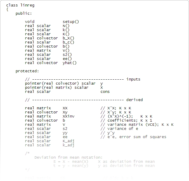
Stata también incluye un lenguaje de programación avanzado: Mata.
Mata tiene las estructuras, punteros y clases que esperas en tu lenguaje de programación y agrega soporte directo para la programación matricial.
Aunque no es necesario programar para usar Stata, es reconfortante saber que un lenguaje de programación rápido y completo es parte integral de Stata. Mata es tanto un entorno interactivo para manipular matrices como un entorno de desarrollo completo que puede producir código compilado y optimizado. Incluye funciones especiales para procesar datos de panel, realiza operaciones con matrices reales o complejas, ofrece soporte completo para programación orientada a objetos y está completamente integrado con todos los aspectos de Stata. Stata también cuenta con una completa integración con Python, lo que permite aprovechar toda la potencia de Python directamente desde el código de Stata.
Stata también tiene PyStata, que proporciona una integración completa con Python, lo que le permite aprovechar todo el poder de Python directamente desde su código Stata y aprovechar todo el poder de Stata desde su código Python.
Stata incluso te permite incorporar complementos de C, C++ y Java en tus programas mediante una API nativa para cada lenguaje. ¡Incluso puedes incrustar código Java directamente en tu código de Stata!

Stata es tan programable que los desarrolladores y usuarios agregan nuevas funciones todos los días para responder a las crecientes demandas de los investigadores actuales.
Con las capacidades de Internet de Stata, se pueden instalar nuevas funciones y actualizaciones oficiales a través de Internet con un solo clic.
Todos los usuarios registrados de la versión actual de Stata (Stata 19) pueden acceder a soporte técnico gratuito. Si aún no ha registrado su copia de Stata, complete el formulario de registro en línea.
Contamos con un equipo dedicado de programadores y estadísticos expertos en Stata para responder a sus preguntas técnicas. Desde soluciones complejas de gestión de datos hasta cómo lograr que su gráfico tenga la apariencia perfecta, y desde la explicación de un error estándar robusto hasta la especificación de su modelo multinivel, tenemos las respuestas.
![]()
Stata funciona en ordenadores Windows, Mac y Linux/Unix; sin embargo, nuestras licencias no son específicas de ninguna plataforma. Esto significa que si tiene una portátil Mac y una de escritorio Windows, no necesita dos licencias independientes para ejecutar Stata. Puede instalar su licencia de Stata en cualquiera de las plataformas compatibles. Los conjuntos de datos, programas y otros datos de Stata se pueden compartir entre plataformas sin necesidad de traducción. También puede importar conjuntos de datos de otros paquetes estadísticos, hojas de cálculo y bases de datos de forma rápida y sencilla.
Utilizado por investigadores durante más de 40 años, Stata proporciona todo lo que necesita para la ciencia de datos: manipulación de datos, visualización, estadísticas e informes automatizados.
Seleccione su disciplina y vea cómo Stata puede trabajar para usted.
Lleve su investigación más lejos con las nuevas funciones de Stata 19.
Stata 19 tiene algo para todos. A continuación, enumeramos los aspectos más destacados de esta versión. Stata 19 es único porque la mayoría de las nuevas funciones pueden ser utilizadas por investigadores de todas las disciplinas.
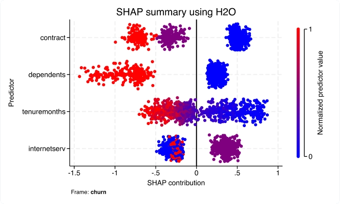
Con la nueva suite h2oml, utilice el aprendizaje automático a través de H2O para extraer información valiosa de los datos cuando los modelos estadísticos tradicionales resultan insuficientes. Los métodos de aprendizaje automático se utilizan a menudo para resolver problemas de investigación y empresariales centrados en la predicción.
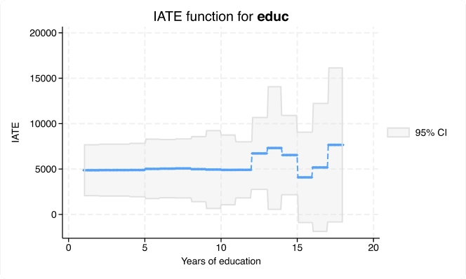
Con el nuevo comando cate, puede ir más allá de estimar un efecto general del tratamiento para estimar efectos individualizados o específicos del grupo que aborden este tipo de preguntas de investigación.
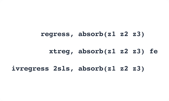
Absorba no solo una sino múltiples variables categóricas de alta dimensión en sus modelos lineales y lineales de efectos fijos con la opción absorb() de los comandos areg y xtreg.
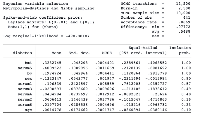
Con el nuevo comando bayesselect, puede realizar la selección bayesiana de variables para la regresión lineal. Este enfoque ofrece una interpretación intuitiva y una inferencia estable, considerando la incertidumbre del modelo.
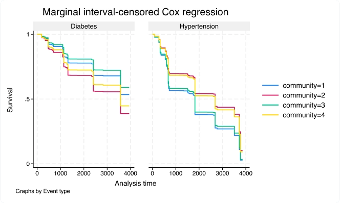
Utilice el nuevo comando stmgintcox para analizar datos de eventos múltiples censurados por intervalo.
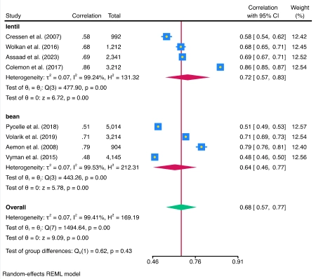
La suite meta ahora admite el metanálisis (MA) de un coeficiente de correlación. Se admiten todas las funciones estándar de metanálisis, como los diagramas de bosque y el análisis de subgrupos.
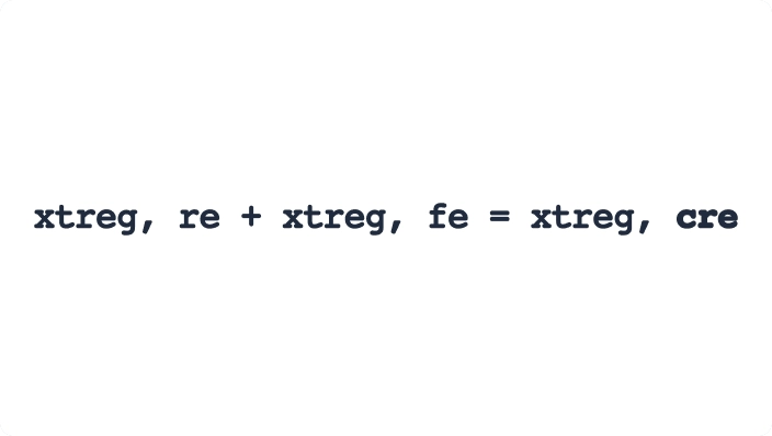
¿Necesita estimaciones de coeficientes de covariables invariantes en el tiempo en su modelo de datos de panel? Con xtreg, cre , ahora puede ajustar un modelo de efectos aleatorios correlacionados.
Con el nuevo comando xtvar, ahora puede ajustar un modelo vectorial autorregresivo (VAR) de datos de panel para analizar las trayectorias de variables relacionadas cuando observa múltiples unidades o paneles a lo largo del tiempo.
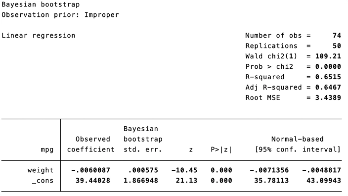
Puede usar el nuevo prefijo bayesboot para realizar un bootstrap bayesiano de las estadísticas generadas por comandos oficiales y aportados por la comunidad. El bootstrap bayesiano puede incorporar información previa para obtener estimaciones de parámetros más precisas.
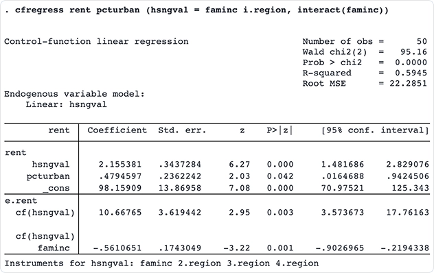
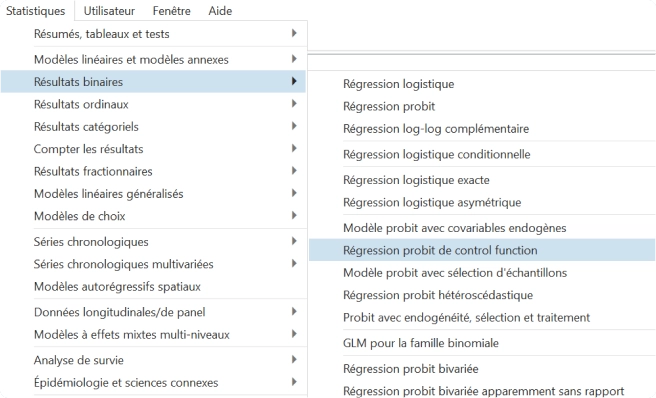
Ajuste modelos lineales y probit de función de control con los nuevos comandos cfregress y cfprobit. Los modelos de función de control ofrecen un enfoque más flexible a los métodos tradicionales de variables instrumentales (VI) al incluir variables endógenas.
El nuevo comando bayes:qreg se ajusta a la regresión cuantil bayesiana. El marco bayesiano proporciona distribuciones posteriores completas para los coeficientes de la regresión cuantil, lo que permite una inferencia exhaustiva.
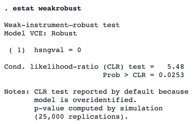
Utilice el nuevo comando estat weakrobust para realizar inferencias confiables en regresores endógenos.
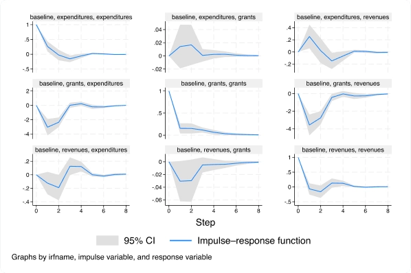
Con el nuevo comando ivsvar, puede utilizar instrumentos en lugar de restricciones de corto plazo para estimar efectos causales dinámicos.
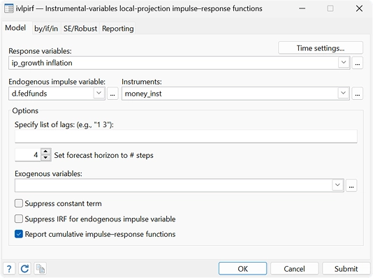
Con el nuevo comando ivlpirf, puede tener en cuenta la endogeneidad al utilizar proyecciones locales para estimar efectos causales dinámicos.

Utilice el nuevo comando de postestimación estat mundlak después de xtreg para elegir entre modelos de efectos aleatorios (RE), efectos fijos (FE) o efectos aleatorios correlacionados (CRE) incluso con errores estándar robustos a grupos, bootstrap o jackknife.
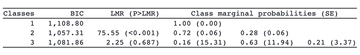
Con el nuevo comando lcstats, puede utilizar estadísticas como la entropía y una variedad de criterios de información para ayudarlo a determinar la cantidad adecuada de clases.
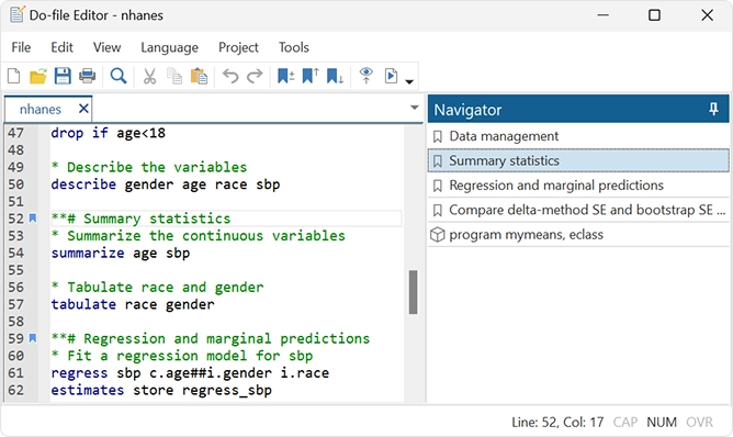
El editor de archivos Do tiene las siguientes novedades: Autocompletado de nombres de variables, macros y resultados almacenados; Mejoras en el plegado de código; Marcadores temporales y permanentes; Plantillas, pestañas y panel de navegación.
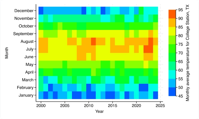
Nuevas características gráficas: Mapas de calor (dos vías); Gráfico de rango y puntos con picos limitados (dos vías); Gráfico de rango y puntos con picos (dos vías); Etiquetado mejorado, CI y control de agrupaciones para gráficos de barras, gráficos de puntos y diagramas de caja; Colores por variable para más gráficos.
Cree y personalice fácilmente tablas con títulos, notas y opciones de exportación. El comando "tabla" es una herramienta flexible para crear tabulaciones, tablas de estadísticas de resumen, tablas de resultados de regresión y más.
Los menús, diálogos y demás elementos de Stata ahora se pueden mostrar en francés. Si el idioma de su ordenador es francés (fr), Stata usará automáticamente la configuración en francés.
Nuevas funciones lanzadas al ritmo de Stata. Con StataNow, siempre tendrás las últimas funciones.
StataNow es una versión de lanzamiento continuo de Stata, que ofrece nuevas funciones tan pronto como están listas y garantiza que los usuarios siempre tengan acceso a la versión más reciente de Stata.
Directamente del desarrollo a ti. Con StataNow, siempre tienes acceso a las últimas funciones.
Las funciones de StataNow están completamente probadas, certificadas, bien documentadas, con control de versiones (si es necesario) y pulidas según nuestra alta calidad habitual. Estas funciones se priorizan en el ciclo de desarrollo para que estén disponibles en cuanto estén listas, de modo que los usuarios puedan aprovecharlas de inmediato. Como siempre, todas las versiones de Stata se actualizan periódicamente con las correcciones y mejoras necesarias. Puede consultar una lista de todas las incorporaciones a Stata y StataNow desde el lanzamiento de Stata 18.
Las nuevas funciones de StataNow se publican continuamente desde la versión actual hasta la siguiente versión principal. No se publican según un calendario preestablecido. Todas las funciones de StataNow están marcadas como tales en el sitio web y la documentación de Stata.
Dado que StataNow es Stata, cuando mencionamos "Stata" en nuestro sitio web y documentación, también nos referimos a "StataNow". Seremos específicos sobre StataNow para las funciones disponibles únicamente en StataNow. Y como StataNow es Stata, está disponible en todas las ediciones (StataNow/MP, StataNow/SE y StataNow/BE) y en todas las plataformas compatibles (Windows, Mac y Linux). En el sitio web y la documentación, generalmente nos referiremos solo a Stata/MP, Stata/SE y Stata/BE para simplificar. Si tiene una licencia de StataNow como la que se describe a continuación, puede entender que esto se refiere a StataNow/MP, StataNow/SE y StataNow/BE.
Todos los titulares de licencias anuales tienen acceso a StataNow, independientemente de si tienen una licencia anual o multianual, o si su institución tiene una licencia de sitio. Puede acceder a las últimas funciones de StataNow simplemente escribiendo "actualizar todo" en la ventana de comandos o solicitando a su administrador del sistema que actualice su Stata. Los usuarios de Stata 19 podrían tener que escribir "actualizar todo" dos veces. La primera actualización le proporcionará un Stata que sabe cómo actualizarse automáticamente a StataNow. La segunda actualización será StataNow. A continuación, escriba "ayuda qué es nuevo" para ver la lista de todas las funciones.
Los nuevos usuarios pueden obtener StataNow en línea, adquiriendo cualquier licencia anual de Stata.
Si tiene un plan de mantenimiento para su licencia, contáctenos para obtener información sobre la nueva descarga y la licencia de StataNow.
Si tiene una licencia perpetua sin mantenimiento o si su mantenimiento o licencia ha caducado, contáctenos para conocer sus opciones.
Al iniciar Stata, verá StataNow en la pantalla de inicio. También puede escribir "about" y verá StataNow en la primera línea.
Análisis de potencia para regresión logística | Publicado en mayo de 2025
Diseñar un estudio eficaz requiere equilibrar la potencia, el tamaño de la muestra y el coste. El nuevo comando "Power Logistic" de Stata le ayuda a determinar el tamaño de muestra óptimo para modelos de regresión logística sin desperdiciar tiempo ni recursos.
El comando "Power Logistic" de Stata calcula el tamaño de la muestra, la potencia o el tamaño del efecto para la prueba de un coeficiente de interés en un modelo de regresión logística. Al igual que con todos los demás métodos de potencia, "Power Logistic" le permite especificar múltiples valores de parámetros y generar automáticamente resultados tabulares y gráficos.
| OS | Windows 10 Macs with Apple Silicon and macOS 10.13 or newer for Macs with Intel processors |
|---|---|
| Processor | Applie Silicon, Intel or AMD processor (Core i3 equivalent or better) |
| Memory | Stata/MP > 4GB, Stata/SE > 2GB, and Stata/BE 1GB |
| Hard Drive | 4GB |
Utilizado por cientos de miles de investigadores durante más de 40 años, Stata proporciona todo lo que necesita para la ciencia de datos: manipulación de datos, visualización, estadísticas e informes reproducibles.
Seleccione su disciplina y vea cómo Stata puede trabajar para usted.
Data wrangling
Scrape data from the web, import it from standard formats, or pull it in via SQL with JDBC or ODBC. Match-merge, link, append, reshape, transpose, sort, filter. Stata handles Unicode, frames (multiple datasets in memory), BLOBs, regular expressions, and more, whether working with hundreds of thousands or even billions of data points.
Automated reporting and customizable tables
Use Markdown to create Word documents and HTML files with embedded Stata code, output, and graphs. Automate Word, PDF, or Excel reports with both high-level export capabilities and low-level fine-grained programmatic access to automate production of the documents your team needs. Customize tables to clearly communicate results, and export your tables to Word, PDF, HTML, LaTeX, Excel, or Markdown.
Visualisation
Create graphs and customize them programmatically or interactively with the Graph Editor. Edits can even be recorded and "replayed" on other graphs for reproducibility. Export to industry standard formats suitable for web (SVG, PNG) or print (PDF, TIFF, EPS, PS).
Programming
Automate your entire workflow with both scripts and full-blown programming features like classes, structures, and pointers. A unique feature of Stata's programming environment is Mata, a fast and compiled matrix programming language. Of course, it has all the advanced matrix operations you need. It also has access to the power of LAPACK. What's more, it has built-in solvers and optimizers to make implementing your own estimator easier. And you can leverage all of Stata's estimation features and other features from within Mata.
PyStata—Python integration
Interact Stata code with Python code. You can seamlessly pass data and results between Stata and Python. You can use Stata within Jupyter Notebook and other IPython environments. You can call Python libraries such as NumPy, matplotlib, Scrapy, scikit-learn, and more from Stata. You can use Stata analyses from within Python.
Interoperability
Connect to external code via Python, Java, and C++ plugins. Write Python or Java code directly within your Stata code. Control Stata via Jupyter Notebook, OLE Automation, or call it in batch mode. Write custom SQL statements with JDBC and ODBC to extract from or populate databases. Access H2O clusters.
Statistics and modeling
Incorporate state-of-the-art statistical models and results in your workflow. Find groups in your data using unsupervised techniques including cluster analysis, principal components, factor analysis, multidimensional scaling, and correspondence analysis. Understand your groups even better using latent class analysis. When your analysis calls for supervised techniques, Stata has flexible nonparametric methods and an array of regression models from linear and logistic models to mixture models. Stata keeps up when your data call for special techniques. You have access to methods that understand and take advantage of the structure in time series, panel data, survival data, complex survey data, spatial data, and multilevel data. Stata provides the most approachable implementations of Bayesian methods and structural equation modeling available anywhere. You can request bootstrap methods for virtually any estimator. When your analysis calls for it, Stata automates other replication methods and simulations.
Reproducibility
Stata is the only software for data science and statistical analysis featuring a comprehensive version control system that ensures your code continues to run, unaltered, even after updates or new versions are released. No need to keep around multiple legacy installations to avoid breaking your system; Stata code from 25 years ago can still be run without modification. Datasets, graphs, scripts, programs, and more are 100% cross-platform and backward compatible.
Lasso
Use lasso and elastic net for model selection and prediction. And when you want to estimate effects and test coefficients for a few variables of interest, inferential methods provide estimates for these variables while using lassos to select from among a potentially large number of control variables. You can even account for endogenous covariates. Whether your goal is model selection, prediction, or inference, you can use Stata's lasso features with your continuous, binary, count, or time-to-event outcomes.
Panel data
Take full advantage of the extra information that panel data provide while simultaneously handling the peculiarities of panel data. Study the time-invariant features within each panel, the relationships across panels, and how outcomes of interest change over time. Fit linear models or nonlinear models for binary, count, ordinal, censored, or survival outcomes with fixed-effects, random-effects, or population-averaged estimators. Fit dynamic models or models with endogeneity.
Time series
Handle the statistical challenges inherent to time-series data—autocorrelations, common factors, autoregressive conditional heteroskedasticity, unit roots, cointegration, and much more. Analyze univariate time series using ARIMA, ARFIMA, Markov-switching models, ARCH and GARCH models, and unobserved-components models. Compare ARIMA or ARFIMA models using AIC, BIC, and HQIC, and select the best number of autoregressive and moving-average terms. Analyze multivariate time series using VAR, structural VAR, VEC, multivariate GARCH, dynamic-factor models, and state-space models. Compute and graph impulse responses. Test for unit roots. Perform Bayesian time-series analysis.
Cross-sectional models
Fit classical linear models of the relationship between a continuous outcome, such as wage, and the determinants of wage, such as education level, age, experience, and economic sector. If your response is binary (for example, employed or unemployed), ordinal (education level), count (number of children), or censored (ticket sales in an existing venue), don't worry. Stata has maximum likelihood estimators—probit, ordered probit, Poisson, tobit, and many others—that estimate the relationship between such outcomes and their determinants. A vast array of tools is available to analyze such models. Predict outcomes and their confidence intervals. Test equality of parameters, or any linear or nonlinear combination of parameters.
Endogeneity and selection
When explanatory variables are related to omitted observable variables, or when they are related to unobservable variables, or when there is selection bias, then causal relationships are confounded and parameter estimates from standard estimators produce inconsistent estimates of the true relationships. Stata can fit consistent models when there is such endogeneity or selection—whether your outcome variable is continuous, binary, count, or ordinal and whether your data are cross-sectional or panel. Stata can even combine endogenous covariates, selection, and treatment effects in the same model.
Causal inference/Treatment effects
Estimate experimental-style causal effects from observational data; for instance, estimate the effect of a job training program on employment or the effect of a subsidy on production. Fit models for continuous, binary, count, fractional, and survival outcomes with binary or multivalued treatments using inverse-probability weighting (IPW), propensity-score matching, nearest-neighbor matching, regression adjustment, or doubly robust estimators. Fit models with exogenous or endogenous treatments. After estimation, test the overlap assumption and covariate balance. Add endogenous covariates and sample selection to some treatment-effects estimators. In the presence of group and time effects, you can use difference-in-differences (DID) and triple-differences (DDD) estimators. In the presence of high-dimensional covariates, you can use lasso. If causal effects are mediated through another variable, use causal mediation with mediate to disentangle direct and indirect effects.
Marginal effects and marginal means
Marginal effects and marginal means let you analyze and visualize the relationships between your outcome variable and your covariates, even when that outcome is binary, count, ordinal, categorical, or censored (tobit). Estimate population-averaged marginal effects or evaluate marginal effects at interesting or representative values of the covariates. Analyze the effect of interactions. You can even trace out the marginal effect over a range of interesting covariate values or covariate interactions. You can do all of this with marginal means (sometimes called potential-outcome means), even when your “mean” is a probability of a positive outcome or a count from a Poisson model. If you have panel data and random effects, these effects are automatically integrated out to provide marginal (that is, population-averaged) effects.
Choice models
Model your discrete choice data. If your outcome is, for instance, a choice to travel by bus, train, car, or airplane, you can fit a conditional logit, multinomial probit, or mixed logit model. Is your outcome instead a ranking of prefered travel methods? Fit a rank-ordered probit or rank-ordered logit model. Regardless of the model fit, you can use the margins to easily interpret the results. Estimate how much wait times at the airport affect the probability of traveling by air or even by train.
GMM
GMM (generalized method of moments) can be used to fit almost any statistical model, including both exactly identified and overidentified estimation problems. Overidentified problems arise when you have endogeneity, correlation in dynamic panels, sample selection, and many other situations. With Stata, you estimate these models by simply writing your moments and enclosing the parameters in curly braces. You can easily fit cross-sectional, time-series, panel-data, or survival-data models and test your overidentifying restrictions.
Demand systems
Fit demand systems to explore consumers' demand for goods and services. Given a budget and a bundle of goods and services, determine the expenditure and price elasticities for these goods. Choose between the Cobb–Douglas system, Stone's linear expenditure system, the translog indirect utility demand system, the almost ideal demand system (AIDS), the quadratic almost ideal demand system (QUAIDS), and others.
Lasso
Use lasso and elastic net for model selection and prediction. And when you want to estimate effects and test coefficients for a few variables of interest, inferential methods provide estimates for these variables while using lassos to select from among a potentially large number of control variables. You can even account for endogenous covariates. Whether your goal is model selection, prediction, or inference, you can use Stata's lasso features with your continuous, binary, count, or time-to-event outcomes.
Programming
Want to program your own commands to perform estimation, perform data management, or implement other new features? Stata is programmable, and thousands of Stata users have implemented and published thousands of community-contributed commands. These commands look and act just like official Stata commands and are easily installed for free over the Internet from within Stata. A unique feature of Stata's programming environment is Mata, a fast and compiled language with support for matrix types. Of course, it has all the advanced matrix operations you need. It also has access to the power of LAPACK. What's more, it has built-in solvers and optimizers to make implementing your own maximum likelihood, GMM, or other estimators easier. And you can leverage all of Stata's estimation and other features from within Mata. Many of Stata's official commands are themselves implemented in Mata.
PyStata - Python integration
Interact Stata code with Python code. You can seamlessly pass data and results between Stata and Python. You can use Stata within Jupyter Notebook and other IPython environments. You can call Python libraries such as NumPy, matplotlib, Scrapy, scikit-learn, and more from Stata. You can use Stata analyses from within Python.
Forecasting
Build multiequation models, and produce forecasts of levels, trends, rates, etc. Whether you have a small model with a few equations or a complete model of the economy with thousands of equations, Stata can help you build that model and produce forecasts. Your model can include both estimated relationships and known identities. You can easily create and compare forecasts under different scenarios, create static and dynamic forecasts, and even estimate stochastic confidence intervals. You can create your model by using an intuitive command syntax or by using the interactive forecasting control panel.
Survival Analysis
Analyze duration outcomes—outcomes measuring the time to an event such as failure or death—using Stata's specialized tools for survival analysis. Account for the complications inherent in survival data, such as sometimes not observing the event (right-, left-, and interval-censoring), individuals entering the study at differing times (delayed entry), and individuals who are not continuously observed throughout the study (gaps). You can estimate and plot the probability of survival over time. Or model survival as a function of covariates using Cox, Weibull, lognormal, and other regression models. Predict hazard ratios, mean survival time, and survival probabilities. Do you have groups of individuals in your study? Adjust for within-group correlation with a random-effects or shared-frailty model. If you have many potential covariates, use lasso cox and elasticnet cox for model selection and prediction.
Bayesian analysis
Perform Bayesian econometrics analysis using one of the Markov chain Monte Carlo (MCMC) methods. You can choose from various supported models, such as panel-data, hierarchical, VAR, and DSGE models, or you can even program your own. Extensive tools are available to check convergence, including multiple chains. Compute posterior mean estimates and credible intervals for model parameters and functions of model parameters. You can perform both interval- and model-based hypothesis testing. Compare models using Bayes factors. Compute model fit using posterior predictive values. Generate predictions and forecasts. If you want to account for model uncertainty in your regression model, use Bayesian model averaging.
Survey methods
Whether your data require a simple weighted adjustment because of differential sampling rates or you have data from a complex multistage survey, Stata's survey features can provide you with correct standard errors and confidence intervals for your inferences. Simply specify the relevant characteristics of your sampling design, such as sampling weights (including weights at multiple stages), clustering (at one, two, or more stages), stratification, and poststratification. After that, most of Stata's estimation commands can adjust their estimates to correct for your sampling design.
Meta-analysis
Combine results of multiple studies to estimate an overall effect. Use forest plots to visualize results. Use subgroup analysis and meta-regression to explore study heterogeneity. Use funnel plots and formal tests to explore publication bias and small-study effects. Use trim-and-fill analysis to assess the impact of publication bias on results. Perform cumulative and leave-one-out meta-analysis. Perform univariate, multilevel, and multivariate meta-analysis. Use the meta suite, or let the Control Panel interface guide you through your entire meta-analysis.
Automated reporting and customizable tables
Stata is designed for reproducible research, including the ability to create dynamic documents incorporating your analysis results. Create Word or PDF files, populate Excel worksheets with results and format them to your liking, and mix Markdown, HTML, Stata results, and Stata graphs, all from within Stata. Create tables that compare regression results or summary statistics, use default styles or apply your own, and export your tables to Word, PDF, HTML, LaTeX, Excel, or Markdown and include them in your reports.
Multilevel mixed-effects models
Whether the groupings in your data arise in a nested fashion (students nested in classrooms and classrooms nested in schools) or in a nonnested fashion (elementary school crossed with middle school), you can fit a multilevel model to account for the lack of independence within these groups. Fit models for continuous, binary, count, ordinal, and survival outcomes. Estimate variances of random intercepts and random coefficients. Compute intraclass correlations. Predict random effects. Estimate relationships that are population averaged over the random effects.
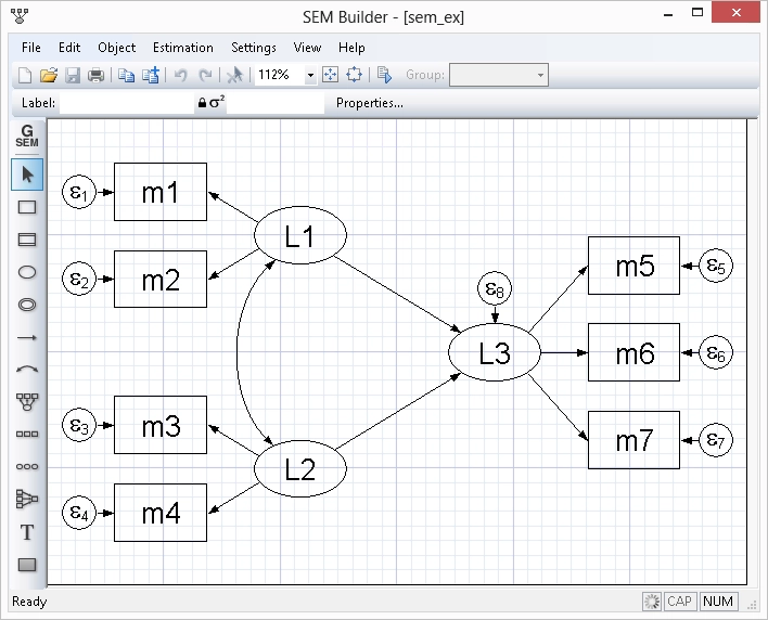
Structural equation modeling (SEM)
Estimate mediation effects, analyze the relationship between an unobserved latent concept such as verbal abilities and the observed variables that measure verbal abilities, or fit a model with complex relationships among both latent and observed variables. Fit models with continuous, binary, count, and ordinal outcomes. Even fit hierarchical models with groups of correlated observations such as children within the same schools. Evaluate model fit. Compute indirect and total effects. Fit models by drawing a path diagram or using the straightforward command syntax.
General Linear Models
Fit one- and two-way models. Or fit models with three, four, or even more factors. Analyze data with nested factors, with fixed and random factors, or with repeated measures. Use ANCOVA models when you have continuous covariates and MANOVA models when you have multiple outcome variables. Further explore the relationships between your outcome and predictors by estimating effect sizes and computing least-squares and marginal means. Perform contrasts and pairwise comparisons. Analyze and plot interactions.
IRT (item response theory)
Explore the relationship between unobserved latent characteristics such as mathematical aptitude and the probability of correctly answering test questions (items). Or explore the relationship between teacher job satisfaction and self-reported responses to questions related to job statisfaction. IRT can be used to create measures of such unobserved traits or place individuals on a scale measuring the trait. It can also be used to select the best items for measuring a latent trait. IRT models are available for binary, graded, rated, partial-credit, and nominal response items. Visualize the relationships using item characteristic curves, and measure overall test performance using test information functions.
Linear, binary and count regressions
Fit classical linear regression models of the relationship between a continuous outcome, such as a reading test score, and the determinants of the score, such as teaching method and the student's reading level in the previous grade. If your response is binary (for example, pass or fail test), ordinal (education level), count (number of students), or categorical (private, public, or home school), don't worry. Stata has maximum likelihood estimators—logistic, ordered logistic, Poisson, multinomial logit, and many others—that estimate the relationship between such outcomes and their determinants. A vast array of tools is available after fitting such models. Predict outcomes and their confidence intervals. Test equality of parameters. Compute linear and nonlinear combinations of parameters.
Linear, binary and count regressions
Account for missing data in your sample using multiple imputation. Choose from univariate and multivariate methods to impute missing values in continuous, censored, truncated, binary, ordinal, categorical, and count variables. Then, in a single step, estimate parameters using the imputed datasets, and combine results. Fit a linear model, logit model, Poisson model, hierarchical model, survival model, or one of the many other supported models. Use the mi command, or let the Control Panel interface guide you through your entire MI analysis.
Choice models
Model your discrete choice data. If your outcome is, for instance, a choice to travel by bus, train, car, or airplane, you can fit a conditional logit, multinomial probit, or mixed logit model. Is your outcome instead a ranking of prefered travel methods? Fit a rank-ordered probit or rank-ordered logit model. Regardless of the model fit, you can use the margins to easily interpret the results. Estimate how much wait times at the airport affect the probability of traveling by air or even by train.
Contrasts, marginal means and profile plots
Quickly and easily obtain contrasts for categorical variables and their interactions. R.edlevel will give you all the contrasts of education level with a reference category. A.edlevel will give you each paired contrast with the next higher education level. There are many more named contrasts, and you can specify your own. If you don't like typing, use a dialog box to select your contrasts. Marginal means are just a simple command or mouse click away after almost any estimation command. Evaluating interaction effects, the effects of moderating variables, is just as easy. And this is not just for linear models, but for models with binary, ordinal, and count outcomes. Even for hierarchical models with correct handling of random effects. A simple command or a few mouse clicks will get you a profile plot of any of these results.
Power, precision and sample size
Before you conduct your experiment, determine the sample size needed to detect meaningful effects without wasting resources. Do you intend to compute CIs for means or variances or perform tests for proportions or correlations? Do you plan to fit a Cox proportional hazards model or compare survivor functions using a log-rank test? Do you want to use a Cochran—Mantel—Haenszel test of association or a Cochran—Armitage trend test? Use Stata's power command to compute power and sample size, create customized tables, and automatically graph the relationships between power, sample size, and effect size for your planned study. Or use the ciwidth command to do the same but for CIs instead of hypothesis tests by computing the required sample size for the desired CI precision. Or use gsdesign to compute stopping boundaries and the required sample sizes for group sequential designs. Instead of commands, use the interactive Control Panel to perform your analysis.
Causal Inference
Estimate experimental-style causal effects from observational data. With Stata's treatment-effects estimators, you can use a potential-outcomes (counterfactuals) framework to estimate, for instance, the effect of family structure on child development or the effect of unemployment on anxiety. Fit models for continuous, binary, count, fractional, and survival outcomes with binary or multivalued treatments using inverse-probability weighting (IPW), propensity-score matching, nearest-neighbor matching, regression adjustment, or doubly robust estimators. If the assignment to a treatment is not independent of the outcome, you can use an endogenous treatment-effects estimator. In the presence of group and time effects, you can use difference-in-differences (DID) and triple-differences (DDD) estimators. In the presence of high-dimensional covariates, you can use lasso. If causal effects are mediated through another variable, use causal mediation with mediate to disentangle direct and indirect effects.
Multivariate methods
Use multivariate analyses to evaluate relationships among variables from many different perspectives. Perform multivariate tests of means, or fit multivariate regression and MANOVA models. Explore relationships between two sets of variables, such as aptitude measurements and achievement measurements, using canonical correlation. Examine the number and structure of latent concepts underlying a set of variables using exploratory factor analysis. Or use principal component analysis to find underlying structure or to reduce the number of variables used in a subsequent analysis. Discover groupings of observations in your data using cluster analysis. If you have known groups in your data, describe differences between them using discriminant analysis.
Automated reporting and customizable tables
Stata is designed for reproducible research, including the ability to create dynamic documents incorporating your analysis results. Create Word or PDF files, populate Excel worksheets with results and format them to your liking, and mix Markdown, HTML, Stata results, and Stata graphs, all from within Stata. Create tables that compare regression results or summary statistics, use default styles or apply your own, and export your tables to Word, PDF, HTML, LaTeX, Excel, or Markdown and include them in your reports.
Bayesian analysis
Perform Bayesian econometrics analysis using one of the Markov chain Monte Carlo (MCMC) methods. You can choose from various supported models, such as panel-data, hierarchical, VAR, and DSGE models, or you can even program your own. Extensive tools are available to check convergence, including multiple chains. Compute posterior mean estimates and credible intervals for model parameters and functions of model parameters. You can perform both interval- and model-based hypothesis testing. Compare models using Bayes factors. Compute model fit using posterior predictive values. Generate predictions and forecasts. If you want to account for model uncertainty in your regression model, use Bayesian model averaging.
Meta-analysis
Combine results of multiple studies to estimate an overall effect. Use forest plots to visualize results. Use subgroup analysis and meta-regression to explore study heterogeneity. Use funnel plots and formal tests to explore publication bias and small-study effects. Use trim-and-fill analysis to assess the impact of publication bias on results. Perform cumulative and leave-one-out meta-analysis. Perform univariate, multilevel, and multivariate meta-analysis. Use the meta suite, or let the Control Panel interface guide you through your entire meta-analysis.
Jupyter Notebook with Stata
Jupyter Notebook is widely used by researchers and scientists to share their ideas and results for collaboration and innovation. It is an easy-to-use web application that allows you to combine code, visualizations, mathematical formulas, narrative text, and other rich media in a single document (a "notebook") for interactive computing and developing. You can invoke Stata and Mata from Jupyter Notebook with the IPython (interactive Python) kernel. This means you can combine the capabilities of both Python and Stata in a single environment to make your work easily reproducible and shareable with others.
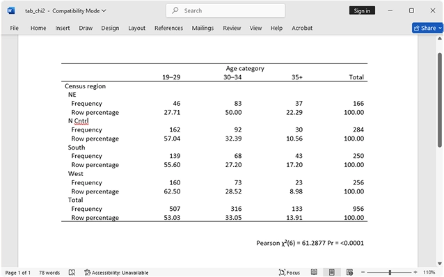
Epidemiological tables
Want to analyze data from a prospectiv321 laddence") study, cohort study, case–control study, or matched case–control study? Stata's tables for epidemiologists make it easy to summarize your data and compute statistics such as incidence-rate ratios, incidence-rate differences, risk ratios, risk differences, odds ratios, and attributable fractions. You can analyze stratified data too—compute Mantel–Haenszel combined estimates, perform tests of homogeneity, and standardize estimates. If you have an ordinal rather than binary exposure, you can perform a test for a trend.
Survival analysis
Analyze duration outcomes—outcomes measuring the time to an event such as failure or death—using Stata's specialized tools for survival analysis. Account for the complications inherent in survival data, such as sometimes not observing the event (right-, left-, and interval-censoring), individuals entering the study at differing times (delayed entry), and individuals who are not continuously observed throughout the study (gaps). You can estimate and plot the probability of survival over time. Or model survival as a function of covariates using Cox, Weibull, lognormal, and other regression models. Predict hazard ratios, mean survival time, and survival probabilities. Do you have groups of individuals in your study? Adjust for within-group correlation with a random-effects or shared-frailty model. If you have many potential covariates, use lasso cox and elasticnet cox for model selection and prediction.
Linear, binary and count regressions
Fit classical ANOVA and linear regression models of the relationship between a continuous outcome, such as weight, and the determinants of weight, such as height, diet, and level of exercise. If your response is binary, ordinal, categorical, or count, don't worry. Stata has estimators for these types of outcomes too. Use logistic regression to adjust odds ratios for confounding variables. Estimate incidence rates using a Poisson model. Analyze matched case–control data with conditional logistic regression. A vast array of tools is available after fitting such models. Predict outcomes and their confidence intervals. Test equality of parameters. Compute linear and nonlinear combinations of parameters.
Survey methods
Whether your data require a simple weighted adjustment because of differential sampling rates or you have data from a complex multistage survey, Stata's survey features can provide you with correct standard errors and confidence intervals for your inferences. Simply specify the relevant characteristics of your sampling design, such as sampling weights (including weights at multiple stages), clustering (at one, two, or more stages), stratification, and poststratification. After that, most of Stata's estimation commands can adjust their estimates to correct for your sampling design.
Marginal means, contrasts and interactions
Marginal means and contrasts let you analyze the relationships between your outcome variable and your predictors, even when your outcome is binary, count, ordinal, or categorical. For instance, after you fit a logistic regression of a disease on an exposure variable and other covariates, your marginal means may be population-averaged risks. Or you can set the covariates to interesting values to compute adjusted risks and then use contrasts to get adjusted risk differences. After fitting almost any model in Stata, you can analyze the effect of covariate interactions and easily create plots to visualize those interactions.
Power, precision and sample size
Before you conduct your experiment, determine the sample size needed to detect meaningful effects without wasting resources. Do you intend to compute CIs for means or variances or perform tests for proportions or correlations? Do you plan to fit a Cox proportional hazards model or compare survivor functions using a log-rank test? Do you want to use a Cochran—Mantel—Haenszel test of association or a Cochran—Armitage trend test? Use Stata's power command to compute power and sample size, create customized tables, and automatically graph the relationships between power, sample size, and effect size for your planned study. Or use the ciwidth command to do the same but for CIs instead of hypothesis tests by computing the required sample size for the desired CI precision. Or use gsdesign to compute stopping boundaries and the required sample sizes for group sequential designs. Instead of commands, use the interactive Control Panel to perform your analysis.
Meta-analysis
Combine results of multiple studies to estimate an overall effect. Use forest plots to visualize results. Use subgroup analysis and meta-regression to explore study heterogeneity. Use funnel plots and formal tests to explore publication bias and small-study effects. Use trim-and-fill analysis to assess the impact of publication bias on results. Perform cumulative and leave-one-out meta-analysis. Perform univariate, multilevel, and multivariate meta-analysis. Use the meta suite, or let the Control Panel interface guide you through your entire meta-analysis.
Causal inference
Estimate experimental-style causal effects from observational data. With Stata's treatment-effects estimators, you can use a potential-outcomes (counterfactuals) framework to estimate, for instance, the effect of family structure on child development or the effect of unemployment on anxiety. Fit models for continuous, binary, count, fractional, and survival outcomes with binary or multivalued treatments using inverse-probability weighting (IPW), propensity-score matching, nearest-neighbor matching, regression adjustment, or doubly robust estimators. If the assignment to a treatment is not independent of the outcome, you can use an endogenous treatment-effects estimator. In the presence of group and time effects, you can use difference-in-differences (DID) and triple-differences (DDD) estimators. In the presence of high-dimensional covariates, you can use lasso. If causal effects are mediated through another variable, use causal mediation with mediate to disentangle direct and indirect effects.
Multiple imputation
Account for missing data in your sample using multiple imputation. Choose from univariate and multivariate methods to impute missing values in continuous, censored, truncated, binary, ordinal, categorical, and count variables. Then, in a single step, estimate parameters using the imputed datasets, and combine results. Fit a linear model, logit model, Poisson model, multilevel model, survival model, or one of the many other supported models. Use the mi command, or let the Control Panel interface guide you through your entire MI analysis.
Multilevel mixed-effects models
Whether the groupings in your data arise in a nested fashion (patients nested in clinics and clinics nested in regions) or in a nonnested fashion (regions crossed with occupations), you can fit a multilevel model to account for the lack of independence within these groups. Fit models for continuous, binary, count, ordinal, and survival outcomes. Estimate variances of random intercepts and random coefficients. Compute intraclass correlations. Predict random effects. Estimate relationships that are population averaged over the random effects.
Bayesian analysis
Fit Bayesian regression models using one of the Markov chain Monte Carlo (MCMC) methods. You can choose from various supported models or even program your own. Extensive tools are available to check convergence, including multiple chains. Compute posterior mean estimates and credible intervals for model parameters and functions of model parameters. You can perform both interval- and model-based hypothesis testing. Compare models using Bayes factors. Compute model fit using posterior predictive values and generate predictions. If you want to account for model uncertainty in your regression model, use Bayesian model averaging.
Additive models of relative risk
Determine how exposures interact to put subjects at a higher risk of experiencing an outcome of interest. For example, you might be investigating how exposure to cigarette smoke and asbestos interact to increase the risk of lung cancer. With Stata's reri command, you can measure two–way interactions in an additive model of relative risk, while accounting for other risk factors. Choose from various supported models, such as binomial generalized linear, Poisson, negative binomial, logistic, Cox, parametric survival, and interval–censored parametric and semiparametric survival models. Estimate the relative excess risk due to interaction (RERI), attributable proportion (AP), and synergy index (SI).
Automated reporting and customizable tables
Stata is designed for reproducible research, including the ability to create dynamic documents incorporating your analysis results. Create Word or PDF files, populate Excel worksheets with results and format them to your liking, and mix Markdown, HTML, Stata results, and Stata graphs, all from within Stata. Create tables that compare regression results or summary statistics, use default styles or apply your own, and export your tables to Word, PDF, HTML, LaTeX, Excel, or Markdown and include them in your reports.
Jupyter Notebook with Stata
Jupyter Notebook is widely used by researchers and scientists to share their ideas and results for collaboration and innovation. It is an easy-to-use web application that allows you to combine code, visualizations, mathematical formulas, narrative text, and other rich media in a single document (a "notebook") for interactive computing and developing. You can invoke Stata and Mata from Jupyter Notebook with the IPython (interactive Python) kernel. This means you can combine the capabilities of both Python and Stata in a single environment to make your work easily reproducible and shareable with others.
Survival analysis
Analyze duration outcomes—outcomes measuring the time to an event such as failure or death—using Stata's specialized tools for survival analysis. Account for the complications inherent in survival data, such as sometimes not observing the event (right-, left-, and interval-censoring), individuals entering the study at differing times (delayed entry), and individuals who are not continuously observed throughout the study (gaps). You can estimate and plot the probability of survival over time. Or model survival as a function of covariates using Cox, Weibull, lognormal, and other regression models. Predict hazard ratios, mean survival time, and survival probabilities. Do you have groups of individuals in your study? Adjust for within-group correlation with a random-effects or shared-frailty model. If you have many potential covariates, use lasso cox and elasticnet cox for model selection and prediction.
Multilevel mixed-effects models
Whether the groupings in your data arise in a nested fashion (patients nested in clinics and clinics nested in regions) or in a nonnested fashion (regions crossed with occupations), you can fit a multilevel model to account for the lack of independence within these groups. Fit models for continuous, binary, count, ordinal, and survival outcomes. Estimate variances of random intercepts and random coefficients. Compute intraclass correlations. Predict random effects. Estimate relationships that are population averaged over the random effects.
Bayesian analysis
Fit Bayesian regression models using one of the Markov chain Monte Carlo (MCMC) methods. You can choose from various supported models or even program your own. Extensive tools are available to check convergence, including multiple chains. Compute posterior mean estimates and credible intervals for model parameters and functions of model parameters. You can perform both interval- and model-based hypothesis testing. Compare models using Bayes factors. Compute model fit using posterior predictive values and generate predictions. If you want to account for model uncertainty in your regression model, use Bayesian model averaging.
Power, precision and sample size
Before you conduct your experiment, determine the sample size needed to detect meaningful effects without wasting resources. Do you intend to compute CIs for means or variances or perform tests for proportions or correlations? Do you plan to fit a Cox proportional hazards model or compare survivor functions using a log-rank test? Do you want to use a Cochran—Mantel—Haenszel test of association or a Cochran—Armitage trend test? Use Stata's power command to compute power and sample size, create customized tables, and automatically graph the relationships between power, sample size, and effect size for your planned study. Or use the ciwidth command to do the same but for CIs instead of hypothesis tests by computing the required sample size for the desired CI precision. Or use gsdesign to compute stopping boundaries and the required sample sizes for group sequential designs. Instead of commands, use the interactive Control Panel to perform your analysis.
Linear, binary and count regressions
Fit classical ANOVA and linear regression models of the relationship between a continuous outcome, such as weight, and the determinants of weight, such as height, diet, and level of exercise. If your response is binary, ordinal, categorical, or count, don't worry. Stata has estimators for these types of outcomes too. Use logistic regression to estimate odds ratios. Estimate incidence rates using a Poisson model. Analyze matched case–control data with conditional logistic regression. A vast array of tools is available after fitting such models. Predict outcomes and their confidence intervals. Test equality of parameters. Compute linear and nonlinear combinations of parameters.
Meta-analysis
Combine results of multiple studies to estimate an overall effect. Use forest plots to visualize results. Use subgroup analysis and meta-regression to explore study heterogeneity. Use funnel plots and formal tests to explore publication bias and small-study effects. Use trim-and-fill analysis to assess the impact of publication bias on results. Perform cumulative and leave-one-out meta-analysis. Perform univariate, multilevel, and multivariate meta-analysis. Use the meta suite, or let the Control Panel interface guide you through your entire meta-analysis.
Multiple imputation
Account for missing data in your sample using multiple imputation. Choose from univariate and multivariate methods to impute missing values in continuous, censored, truncated, binary, ordinal, categorical, and count variables. Then, in a single step, estimate parameters using the imputed datasets, and combine results. Fit a linear model, logit model, Poisson model, hierarchical model, survival model, or one of the many other supported models. Use the mi command, or let the Control Panel interface guide you through your entire MI analysis.
Marginal means, contrasts and interactions
Marginal means and contrasts let you analyze the relationships between your outcome variable and your covariates, even when that outcome is binary, count, ordinal, categorical, or survival. Compute adjusted predictions with covariates set to interesting or representative values. Or compute marginal means for each level of a categorical covariate. Make comparisons of the adjusted predictions or marginal means using contrasts. If you have multilevel data and random effects, these effects are automatically integrated out to provide marginal (that is, population-averaged) estimates. After fitting almost any model in Stata, analyze the effect of covariate interactions, and easily create plots to visualize those interactions.
Causal inference
Estimate experimental-style causal effects from observational data. With Stata's treatment-effects estimators, you can use a potential-outcomes (counterfactuals) framework to estimate, for instance, the effect of family structure on child development or the effect of unemployment on anxiety. Fit models for continuous, binary, count, fractional, and survival outcomes with binary or multivalued treatments using inverse-probability weighting (IPW), propensity-score matching, nearest-neighbor matching, regression adjustment, or doubly robust estimators. If the assignment to a treatment is not independent of the outcome, you can use an endogenous treatment-effects estimator. In the presence of group and time effects, you can use difference-in-differences (DID) and triple-differences (DDD) estimators. In the presence of high-dimensional covariates, you can use lasso. If causal effects are mediated through another variable, use causal mediation with mediate to disentangle direct and indirect effects.
Epidemiological tables
Want to analyze data from a prospective (incidence) study, cohort study, case–control study, or matched case–control study? Stata's tables for epidemiologists make it easy to summarize your data and compute statistics such as incidence-rate ratios, incidence-rate differences, risk ratios, risk differences, odds ratios, and attributable fractions. You can analyze stratified data too—compute Mantel–Haenszel combined estimates, perform tests of homogeneity, and standardize estimates. If you have an ordinal rather than binary exposure, you can perform a test for a trend.
Programming
Want to program your own commands to perform estimation, perform data management, or implement other new features? Stata is programmable, and thousands of Stata users have implemented and published thousands of community-contributed commands. These commands look and act just like official Stata commands and are easily installed for free over the Internet from within Stata. A unique feature of Stata's programming environment is Mata, a fast and compiled language with support for matrix types. Of course, it has all the advanced matrix operations you need. It also has access to the power of LAPACK. What's more, it has built-in solvers and optimizers to make implementing your own maximum likelihood, GMM, or other estimators easier. And you can leverage all of Stata's estimation and other features from within Mata. Many of Stata's official commands are themselves implemented in Mata.
PyStata - Python integration
Interact Stata code with Python code. You can seamlessly pass data and results between Stata and Python. You can use Stata within Jupyter Notebook and other IPython environments. You can call Python libraries such as NumPy, matplotlib, Scrapy, scikit-learn, and more from Stata. You can use Stata analyses from within Python.
Automated reporting and customizable tables
Stata is designed for reproducible research, including the ability to create dynamic documents incorporating your analysis results. Create Word or PDF files, populate Excel worksheets with results and format them to your liking, and mix Markdown, HTML, Stata results, and Stata graphs, all from within Stata. Create tables that compare regression results or summary statistics, use default styles or apply your own, and export your tables to Word, PDF, HTML, LaTeX, Excel, or Markdown and include them in your reports.
General linear models
Fit one- and two-way models. Or fit models with three, four, or even more factors. Analyze data with nested factors, with fixed and random factors, or with repeated measures. Use ANCOVA models when you have continuous covariates and MANOVA models when you have multiple outcome variables. Further explore the relationships between your outcome and predictors by estimating effect sizes and computing least-squares and marginal means. Perform contrasts and pairwise comparisons. Analyze and plot interactions.
Linear, binary and count regressions
Fit classical ANOVA and linear regression models of the relationship between a continuous outcome, such as weight, and the determinants of weight, such as height, diet, and level of exercise. If your response is binary, ordinal, categorical, or count, don't worry. Stata has estimators for these types of outcomes too. Use logistic regression to estimate odds ratios. Estimate incidence rates using a Poisson model. Analyze matched case–control data with conditional logistic regression. A vast array of tools is available after fitting such models. Predict outcomes and their confidence intervals. Test equality of parameters. Compute linear and nonlinear combinations of parameters.
Power, precision and sample size
Before you conduct your experiment, determine the sample size needed to detect meaningful effects without wasting resources. Do you intend to compute CIs for means or variances or perform tests for proportions or correlations? Do you plan to fit a Cox proportional hazards model or compare survivor functions using a log-rank test? Do you want to use a Cochran—Mantel—Haenszel test of association or a Cochran—Armitage trend test? Use Stata's power command to compute power and sample size, create customized tables, and automatically graph the relationships between power, sample size, and effect size for your planned study. Or use the ciwidth command to do the same but for CIs instead of hypothesis tests by computing the required sample size for the desired CI precision. Or use gsdesign to compute stopping boundaries and the required sample sizes for group sequential designs. Instead of commands, use the interactive Control Panel to perform your analysis.
Marginal means, contrasts and interactions
Marginal means and contrasts let you analyze the relationships between your outcome variable and your covariates, even when that outcome is binary, count, ordinal, categorical, or survival. Compute adjusted predictions with covariates set to interesting or representative values. Or compute marginal means for each level of a categorical covariate. Make comparisons of the adjusted predictions or marginal means using contrasts. If you have multilevel data and random effects, these effects are automatically integrated out to provide marginal (that is, population-averaged) estimates. After fitting almost any model in Stata, analyze the effect of covariate interactions, and easily create plots to visualize those interactions.
Multilevel mixed-effects models
Whether the groupings in your data arise in a nested fashion (patients nested in clinics and clinics nested in regions) or in a nonnested fashion (regions crossed with occupations), you can fit a multilevel model to account for the lack of independence within these groups. Fit models for continuous, binary, count, ordinal, and survival outcomes. Estimate variances of random intercepts and random coefficients. Compute intraclass correlations. Predict random effects. Estimate relationships that are population averaged over the random effects.
Meta-analysis
Combine results of multiple studies to estimate an overall effect. Use forest plots to visualize results. Use subgroup analysis and meta-regression to explore study heterogeneity. Use funnel plots and formal tests to explore publication bias and small-study effects. Use trim-and-fill analysis to assess the impact of publication bias on results. Perform cumulative and leave-one-out meta-analysis. Perform univariate, multilevel, and multivariate meta-analysis. Use the meta suite, or let the Control Panel interface guide you through your entire meta-analysis.
Multiple imputation
Account for missing data in your sample using multiple imputation. Choose from univariate and multivariate methods to impute missing values in continuous, censored, truncated, binary, ordinal, categorical, and count variables. Then, in a single step, estimate parameters using the imputed datasets, and combine results. Fit a linear model, logit model, Poisson model, hierarchical model, survival model, or one of the many other supported models. Use the mi command, or let the Control Panel interface guide you through your entire MI analysis.
Survival analysis
Analyze duration outcomes—outcomes measuring the time to an event such as failure or death—using Stata's specialized tools for survival analysis. Account for the complications inherent in survival data, such as sometimes not observing the event (right-, left-, and interval-censoring), individuals entering the study at differing times (delayed entry), and individuals who are not continuously observed throughout the study (gaps). You can estimate and plot the probability of survival over time. Or model survival as a function of covariates using Cox, Weibull, lognormal, and other regression models. Predict hazard ratios, mean survival time, and survival probabilities. Do you have groups of individuals in your study? Adjust for within-group correlation with a random-effects or shared-frailty model. If you have many potential covariates, use lasso cox and elasticnet cox for model selection and prediction.
Epidemiological tables
Want to analyze data from a prospective (incidence) study, cohort study, case–control study, or matched case–control study? Stata's tables for epidemiologists make it easy to summarize your data and compute statistics such as incidence-rate ratios, incidence-rate differences, risk ratios, risk differences, odds ratios, and attributable fractions. You can analyze stratified data too—compute Mantel–Haenszel combined estimates, perform tests of homogeneity, and standardize estimates. If you have an ordinal rather than binary exposure, you can perform a test for a trend.
Additive models of relative risk
Determine how exposures interact to put subjects at a higher risk of experiencing an outcome of interest. For example, you might be investigating how exposure to cigarette smoke and asbestos interact to increase the risk of lung cancer. With Stata's reri command, you can measure two–way interactions in an additive model of relative risk, while accounting for other risk factors. Choose from various supported models, such as binomial generalized linear, Poisson, negative binomial, logistic, Cox, parametric survival, and interval–censored parametric and semiparametric survival models. Estimate the relative excess risk due to interaction (RERI), attributable proportion (AP), and synergy index (SI).
Automated reporting and customizable tables
Stata is designed for reproducible research, including the ability to create dynamic documents incorporating your analysis results. Create Word or PDF files, populate Excel worksheets with results and format them to your liking, and mix Markdown, HTML, Stata results, and Stata graphs, all from within Stata. Create tables that compare regression results or summary statistics, use default styles or apply your own, and export your tables to Word, PDF, HTML, LaTeX, Excel, or Markdown and include them in your reports.
Jupyter Notebook with Stata
Jupyter Notebook is widely used by researchers and scientists to share their ideas and results for collaboration and innovation. It is an easy-to-use web application that allows you to combine code, visualizations, mathematical formulas, narrative text, and other rich media in a single document (a "notebook") for interactive computing and developing. You can invoke Stata and Mata from Jupyter Notebook with the IPython (interactive Python) kernel. This means you can combine the capabilities of both Python and Stata in a single environment to make your work easily reproducible and shareable with others.
Survey methods
Whether your data require a simple weighted adjustment because of differential sampling rates or you have data from a complex multistage survey, Stata's survey features can provide you with correct standard errors and confidence intervals for your inferences. Simply specify the relevant characteristics of your sampling design, such as sampling weights (including weights at multiple stages), clustering (at one, two, or more stages), stratification, and poststratification. After that, most of Stata's estimation commands can adjust their estimates to correct for your sampling design.
Multiple imputation
Account for missing data in your sample using multiple imputation. Choose from univariate and multivariate methods to impute missing values in continuous, censored, truncated, binary, ordinal, categorical, and count variables. Then, in a single step, estimate parameters using the imputed datasets, and combine results. Fit a linear model, logit model, Poisson model, multilevel model, survival model, or one of the many other supported models. Use the mi command, or let the Control Panel interface guide you through your entire MI analysis.
Multilevel mixed-effects models
Whether the groupings in your data arise in a nested fashion (students nested in schools and schools nested in districts) or in a nonnested fashion (regions crossed with occupations), you can fit a multilevel model to account for the lack of independence within these groups. Fit models for continuous, binary, count, ordinal, and survival outcomes. Estimate variances of random intercepts and random coefficients. Compute intraclass correlations. Predict random effects. Estimate relationships that are population averaged over the random effects.
Panel data
Take full advantage of the extra information that panel data provide while simultaneously handling the peculiar difficulties that panel data present. Study the time-invariant idiosyncratic features within each panel, the relationships across panels, and how outcomes of interest change over time. Fit linear models or nonlinear models for binary, count, ordinal, censored, or survival outcomes with fixed-effects, random-effects, or population-averaged estimators. Fit dynamic models or models with endogeneity. Fit Bayesian panel-data models.
Meta-analysis
Combine results of multiple studies to estimate an overall effect. Use forest plots to visualize results. Use subgroup analysis and meta-regression to explore study heterogeneity. Use funnel plots and formal tests to explore publication bias and small-study effects. Use trim-and-fill analysis to assess the impact of publication bias on results. Perform cumulative and leave-one-out meta-analysis. Perform univariate, multilevel, and multivariate meta-analysis. Use the meta suite, or let the Control Panel interface guide you through your entire meta-analysis.
Linear, binary and count regressions
Fit classical linear models of the relationship between a continuous outcome, such as wage, and the determinants of wage, such as education level, age, experience, and economic sector. If your response is binary (for example, employed or unemployed), ordinal (education level), or count (number of children), don't worry. Stata has maximum likelihood estimators—probit, ordered probit, Poisson, and many others—that estimate the relationship between such outcomes and their determinants. A vast array of tools is available to analyze such models. Predict outcomes and their confidence intervals. Test equality of parameters or any linear or nonlinear combination of parameters.
Structural equation modeling (SEM)
Estimate mediation effects, analyze the relationship between an unobserved latent concept such as a person's level of conservatism and the observed variables that measure conservatism, model a system with many endogenous variables and correlated errors, or fit a model with complex relationships among both latent and observed variables. Fit models with continuous, binary, count, ordinal, fractional, and survival outcomes. Even fit multilevel models with groups of correlated observations such as children within the same schools. Evaluate model fit. Compute indirect and total effects. Fit models by drawing a path diagram or using the straightforward command syntax.
Adjusted predictions, interactions and moderation
Adjusted predictions and marginal means let you analyze the relationships between your outcome variable and your covariates, even when that outcome is binary, count, ordinal, or categorical. Compute adjusted predictions with covariates set to interesting or representative values. Or compute marginal means for each level of a categorical covariate. Make comparisons of the adjusted predictions or marginal means using contrasts. If you have multilevel or panel data and random effects, these effects are automatically integrated out to provide marginal (that is, population-averaged) estimates. After fitting almost any model in Stata, analyze the effect of moderating variables, and easily create interaction plots.
Choice Models
Model your discrete choice data. If your outcome is, for instance, high-school graduates' choices to attend college, attend a trade school, or to work, you can fit a conditional logit, multinomial probit, or mixed logit model. Is your outcome instead a ranking of prefered alternatives? Fit a rank-ordered probit or rank-ordered logit model. Regardless of the model fit, you can use the margins to easily interpret the results. Estimate how much distance to the nearest college affects the probability of enrolling in college and even the probability of going to a trade school.
Bayesian analysis
Fit Bayesian regression models using one of the Markov chain Monte Carlo (MCMC) methods. You can choose from various supported models or even program your own. Extensive tools are available to check convergence, including multiple chains. Compute posterior mean estimates and credible intervals for model parameters and functions of model parameters. You can perform both interval- and model-based hypothesis testing. Compare models using Bayes factors. Compute model fit using posterior predictive values and generate predictions. If you want to account for model uncertainty in your regression model, use Bayesian model averaging.
Causal inference
Estimate experimental-style causal effects from observational data. With Stata's treatment-effects estimators, you can use a potential-outcomes (counterfactuals) framework to estimate, for instance, the effect of family structure on child development or the effect of unemployment on anxiety. Fit models for continuous, binary, count, fractional, and survival outcomes with binary or multivalued treatments using inverse-probability weighting (IPW), propensity-score matching, nearest-neighbor matching, regression adjustment, or doubly robust estimators. If the assignment to a treatment is not independent of the outcome, you can use an endogenous treatment-effects estimator. In the presence of group and time effects, you can use difference-in-differences (DID) and triple-differences (DDD) estimators. In the presence of high-dimensional covariates, you can use lasso. If causal effects are mediated through another variable, use causal mediation with mediate to disentangle direct and indirect effects.
Programming
Want to program your own commands to perform estimation, perform data management, or implement other new features? Stata is programmable, and thousands of Stata users have implemented and published thousands of community-contributed commands. These commands look and act just like official Stata commands and are easily installed for free over the Internet from within Stata. A unique feature of Stata's programming environment is Mata, a fast and compiled language with support for matrix types. Of course, it has all the advanced matrix operations you need. It also has access to the power of LAPACK. What's more, it has built-in solvers and optimizers to make implementing your own maximum likelihood, GMM, or other estimators easier. And you can leverage all of Stata's estimation and other features from within Mata. Many of Stata's official commands are themselves implemented in Mata.
Automated reporting and customizable tables
Stata is designed for reproducible research, including the ability to create dynamic documents incorporating your analysis results. Create Word or PDF files, populate Excel worksheets with results and format them to your liking, and mix Markdown, HTML, Stata results, and Stata graphs, all from within Stata. Create tables that compare regression results or summary statistics, use default styles or apply your own, and export your tables to Word, PDF, HTML, LaTeX, Excel, or Markdown and include them in your reports.
Jupyter Notebook with Stata
Jupyter Notebook is widely used by researchers and scientists to share their ideas and results for collaboration and innovation. It is an easy-to-use web application that allows you to combine code, visualizations, mathematical formulas, narrative text, and other rich media in a single document (a "notebook") for interactive computing and developing. You can invoke Stata and Mata from Jupyter Notebook with the IPython (interactive Python) kernel. This means you can combine the capabilities of both Python and Stata in a single environment to make your work easily reproducible and shareable with others.
Survey methods
Whether your data require a simple weighted adjustment because of differential sampling rates or you have data from a complex multistage survey, Stata's survey features can provide you with correct standard errors and confidence intervals for your inferences. Simply specify the relevant characteristics of your sampling design, such as sampling weights (including weights at multiple stages), clustering (at one, two, or more stages), stratification, and poststratification. After that, most of Stata's estimation commands can adjust their estimates to correct for your sampling design.
Multilevel mixed-effects models
Whether the groupings in your data arise in a nested fashion (patients nested in clinics and clinics nested in regions) or in a nonnested fashion (regions crossed with occupations), you can fit a multilevel model to account for the lack of independence within these groups. Fit models for continuous, binary, count, ordinal, and survival outcomes. Estimate variances of random intercepts and random coefficients. Compute intraclass correlations. Predict random effects. Estimate relationships that are population averaged over the random effects.
Panel data
Take full advantage of the extra information that panel data provide while simultaneously handling the peculiarities of panel data. Study the time-invariant features within each panel, the relationships across panels, and how outcomes of interest change over time. Fit linear models or nonlinear models for binary, count, ordinal, censored, or survival outcomes with fixed-effects, random-effects, or population-averaged estimators. Fit dynamic models or models with endogeneity. Fit Bayesian panel-data models.
Structural equation modeling (SEM)
Estimate mediation effects, analyze the relationship between an unobserved latent concept such as depression and the observed variables that measure depression, model a system with many endogenous variables and correlated errors, or fit a model with complex relationships among both latent and observed variables. Fit models with continuous, binary, count, ordinal, fractional, and survival outcomes. Even fit multilevel models with groups of correlated observations such as children within the same schools. Evaluate model fit. Compute indirect and total effects. Fit models by drawing a path diagram or using the straightforward command syntax.
Linear, binary and count regressions
Fit classical linear models of the relationship between a continuous outcome, such as wage, and the determinants of wage, such as education level, age, experience, and economic sector. If your response is binary (for example, employed or unemployed), ordinal (education level), or count (number of children), don't worry. Stata has maximum likelihood estimators—probit, ordered probit, Poisson, and many others—that estimate the relationship between such outcomes and their determinants. A vast array of tools is available to analyze such models. Predict outcomes and their confidence intervals. Test equality of parameters or any linear or nonlinear combination of parameters.
Meta-analysis
Combine results of multiple studies to estimate an overall effect. Use forest plots to visualize results. Use subgroup analysis and meta-regression to explore study heterogeneity. Use funnel plots and formal tests to explore publication bias and small-study effects. Use trim-and-fill analysis to assess the impact of publication bias on results. Perform cumulative and leave-one-out meta-analysis. Perform univariate, multilevel, and multivariate meta-analysis. Use the meta suite, or let the Control Panel interface guide you through your entire meta-analysis.
Multiple imputation
Account for missing data in your sample using multiple imputation. Choose from univariate and multivariate methods to impute missing values in continuous, censored, truncated, binary, ordinal, categorical, and count variables. Then, in a single step, estimate parameters using the imputed datasets, and combine results. Fit a linear model, logit model, Poisson model, hierarchical model, survival model, or one of the many other supported models. Use the mi command, or let the Control Panel interface guide you through your entire MI analysis.
Adjusted predictions, contrasts and interactions
Adjusted predictions and contrasts let you analyze the relationships between your outcome variable and your covariates, even when that outcome is binary, count, ordinal, or categorical. Compute adjusted predictions with covariates set to interesting or representative values. Or compute marginal means for each level of a categorical covariate. Make comparisons of the adjusted predictions or marginal means using contrasts. If you have multilevel or panel data and random effects, these effects are automatically integrated out to provide marginal (that is, population-averaged) estimates. After fitting almost any model in Stata, analyze the effect of covariate interactions, and easily create plots to visualize those interactions.
Survival analysis
Analyze duration outcomes—outcomes measuring the time to an event such as failure or death—using Stata's specialized tools for survival analysis. Account for the complications inherent in survival data, such as sometimes not observing the event (right-, left-, and interval-censoring), individuals entering the study at differing times (delayed entry), and individuals who are not continuously observed throughout the study (gaps). You can estimate and plot the probability of survival over time. Or model survival as a function of covariates using Cox, Weibull, lognormal, and other regression models. Predict hazard ratios, mean survival time, and survival probabilities. Do you have groups of individuals in your study? Adjust for within-group correlation with a random-effects or shared-frailty model. If you have many potential covariates, use lasso cox and elasticnet cox for model selection and prediction.
Causal inference
Estimate experimental-style causal effects from observational data. With Stata's treatment-effects estimators, you can use a potential-outcomes (counterfactuals) framework to estimate, for instance, the effect of family structure on child development or the effect of unemployment on anxiety. Fit models for continuous, binary, count, fractional, and survival outcomes with binary or multivalued treatments using inverse-probability weighting (IPW), propensity-score matching, nearest-neighbor matching, regression adjustment, or doubly robust estimators. If the assignment to a treatment is not independent of the outcome, you can use an endogenous treatment-effects estimator. In the presence of group and time effects, you can use difference-in-differences (DID) and triple-differences (DDD) estimators. In the presence of high-dimensional covariates, you can use lasso. If causal effects are mediated through another variable, use causal mediation with mediate to disentangle direct and indirect effects.
Time Series
Handle the statistical challenges inherent to time-series data—autocorrelations, common factors, autoregressive conditional heteroskedasticity, unit roots, cointegration, and much more. Analyze univariate time series using ARIMA, ARFIMA, Markov-switching models, ARCH and GARCH models, and unobserved-components models. Analyze multivariate time series using VAR, structural VAR, VEC, multivariate GARCH, dynamic-factor models, and state-space models. Compute and graph impulse responses. Test for unit roots. Perform Bayesian time-series analysis.
IRT (item response theory)
Explore the relationship between unobserved latent characteristics such as hospital satisfaction and the probability of responding positively to questionnaire items related to satisfaction. Or explore the relationship between unobserved health and self-reported responses to questions about mobility, independence, and other health-affected activities. IRT can be used to create measures of such unobserved traits or place individuals on a scale measuring the trait. It can also be used to select the best items for measuring a latent trait. IRT models are available for binary, graded, rated, partial-credit, and nominal response items. Visualize the relationships using item characteristic curves, and measure overall test performance using test information functions.
Automated reporting and customizable tables
Stata is designed for reproducible research, including the ability to create dynamic documents incorporating your analysis results. Create Word or PDF files, populate Excel worksheets with results and format them to your liking, and mix Markdown, HTML, Stata results, and Stata graphs, all from within Stata. Create tables that compare regression results or summary statistics, use default styles or apply your own, and export your tables to Word, PDF, HTML, LaTeX, Excel, or Markdown and include them in your reports.
Jupyter Notebook with Stata
Jupyter Notebook is widely used by researchers and scientists to share their ideas and results for collaboration and innovation. It is an easy-to-use web application that allows you to combine code, visualizations, mathematical formulas, narrative text, and other rich media in a single document (a "notebook") for interactive computing and developing. You can invoke Stata and Mata from Jupyter Notebook with the IPython (interactive Python) kernel. This means you can combine the capabilities of both Python and Stata in a single environment to make your work easily reproducible and shareable with others.


Este sitio web utiliza cookies para mejorar su experiencia mientras navega por el sitio. De estas cookies, las que se clasifican como necesarias se almacenan en su navegador, ya que son esenciales para el funcionamiento básico del sitio web. También utilizamos cookies de terceros que nos ayudan a analizar y comprender cómo utiliza este sitio web. Estas cookies solo se almacenarán en su navegador con su consentimiento. También tiene la opción de rechazar estas cookies. Sin embargo, rechazar algunas de ellas puede afectar su experiencia de navegación.
| Name | Description | Lifetime |
|---|---|---|
| ADD_TO_CART | (Adobe Commerce only) Used by Google Tag Manager | 1 Year |
| GUEST-VIEW | Stores the Order ID that guest shoppers use to retrieve their order status. Guest orders view. Used in Orders and Returns widgets | 1 Year |
| LOGIN_REDIRECT | Preserves the destination page that was loading before the customer was directed to log in | 1 Year |
| MAGE-BANNERS-CACHE-STORAGE | (Adobe Commerce only) Stores banner content locally to improve performance | 1 Year |
| MAGE-MESSAGES | Tracks error messages and other notifications that are shown to the user | 1 Year |
| MAGE-TRANSLATION-STORAGE | Stores translated content when requested by the shopper | 1 Year |
| MAGE-TRANSLATION-FILE-VERSION | Tracks the version of translations in local storage | 1 Year |
| PRODUCT_DATA_STORAGE | Stores configuration for product data related to Recently Viewed/Compared Products | 1 Year |
| RECENTLY_COMPARED_PRODUCT | Stores product IDs of recently compared products | 1 Year |
| RECENTLY_COMPARED_PRODUCT_PREVIOUS | Stores product IDs of previously compared products for easy navigation | 1 Year |
| RECENTLY_VIEWED_PRODUCT | Stores product IDs of recently viewed products for easy navigation | 1 Year |
| RECENTLY_VIEWED_PRODUCT_PREVIOUS | Stores product IDs of recently previously viewed products for easy navigation | 1 Year |
| REMOVE_FROM_CART | (Adobe Commerce only) Used by Google Tag Manager | 1 Year |
| STF | Records the time messages are sent by the SendFriend | 1 Year |
| X-MAGENTO-VARY | Configuration setting that improves performance when using Varnish static content caching | 1 Year |
| FORM_KEY | A security measure that appends a random string to all form submissions to protect the data from Cross-Site Request Forgery | 1 Year |
| MAGE-CACHE-SESSID | The value of this cookie triggers the cleanup of local cache storage | 1 Year |
| MAGE-CACHE-STORAGE | Local storage of visitor-specific content that enables ecommerce functions | 1 Year |
| MAGE-CACHE-STORAGE-SECTION-INVALIDATION | Forces local storage of specific content sections that should be invalidated | 1 Year |
| PERSISTENT_SHOPPING_CART | Stores the key (ID) of persistent cart to make it possible to restore the cart for an anonymous shopper | 1 Year |
| PRIVATE_CONTENT_VERSION | Appends a random, unique number and time to pages with customer content to prevent them from being cached on the server | 1 Year |
| SECTION_DATA_IDS | Stores customer-specific information related to shopper-initiated actions, such as wish list display and checkout information | 1 Year |
| STORE | Tracks the specific store view/locale selected by the shopper | 1 Year |
| Name | Description | Lifetime |
|---|---|---|
| CUSTOMER_SEGMENT_IDS | Stores your Customer Segment ID | 1 Year |
| EXTERNAL_NO_CACHE | A flag that, indicates whether caching is on or off | 1 Year |
| FRONTEND | Your session ID on the server | 1 Year |
| GUEST-VIEW | Allows guests to edit their orders | 1 Year |
| LAST_CATEGORY | The last category you visited | 1 Year |
| LAST_PRODUCT | The last product you looked at | 1 Year |
| NEWMESSAGE | Indicates whether a new message has been received | 1 Year |
| NO_CACHE | Indicates whether it is allowed to use cache | 1 Year |
| Name | Description | Lifetime |
|---|---|---|
| MG_DNT | Allows you to restrict Adobe Commerce data collection if you have custom code to manage cookie consent on your site | 1 Year |
| USER_ALLOWED_SAVE_COOKIE | Used for cookie restriction mode | 1 Year |
| AUTHENTICATION_FLAG | Indicates if a shopper has signed in or signed out | 1 Year |
| DATASERVICES_CUSTOMER_ID | Indicates if a shopper has signed in or signed out | 1 Year |
| DATASERVICES_CUSTOMER_GROUP | Indicates a customer's group. This cookie is stored as sha1 checksum of the customer's group ID | 1 Year |
| DATASERVICES_CART_ID | Identifies a shopper's cart actions | 1 Year |
| DATASERVICES_PRODUCT_CONTEXT | Identifies a shopper's product interactions. This cookie contains the customer's unique quote ID in the system | 1 Year |
| Name | Description | Lifetime |
|---|---|---|
| _ga | Used by Google Analytics | 1 Year |
| _ga_* | Used by Google Analytics | 1 Year |


Validate your login
Registrarse
Crear una nueva cuenta