
Explore. Visualise. Model. Better insight starts with Stata
Fast. Accurate. Easy to use. Stata is a complete, integrated software package that provides all your data science needs—data manipulation, visualisation, statistics, and automated reporting.
Purchase or Upgrade your Stata
Whats new in Stata 19
Purchase or Upgrade your Stata
Buy Stata for business, government, nonprofit, educational, or student use.
Choose the appropriate license type (student, academic, business, etc.) and specify whether you are purchasing, upgrading, or renewing your software. The available options will adjust according to your selections.
| OS | Windows 10 Macs with Apple Silicon and macOS 10.13 or later for Macs with Intel processors |
|---|---|
| Processor | Apple Silicon, Intel or AMD Processor (Core i3 or higher) |
| Memory | 4GB RAM |
| Hard Drive | 2GB |
| Graphics | ATI Radeon 8500 or Nvidia GeForce 4 or higher video card |
Data Management
Statistics
Graphics
Why Stata?
Fast. Accurate. Easy to use. Stata is a complete, integrated software package that provides all your data science needs—data manipulation, visualization, statistics, and automated reporting.
|
|
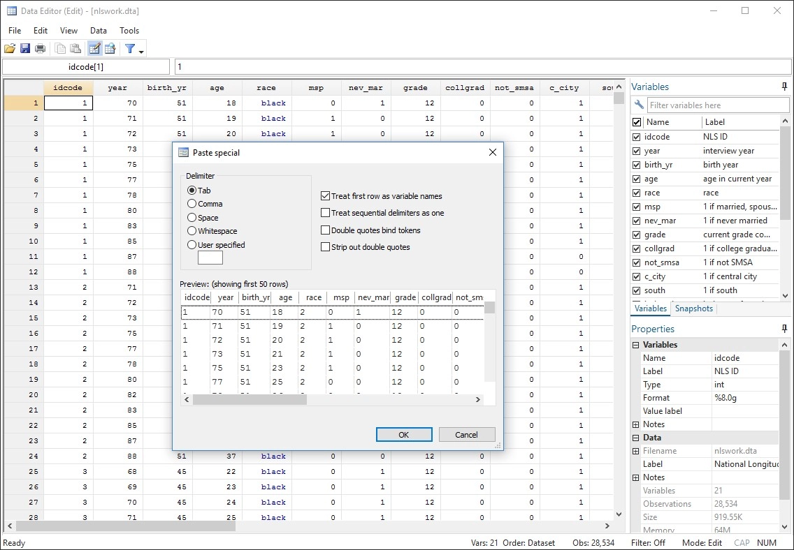
Master your Data
Stata's data management features give you complete control.
|
|
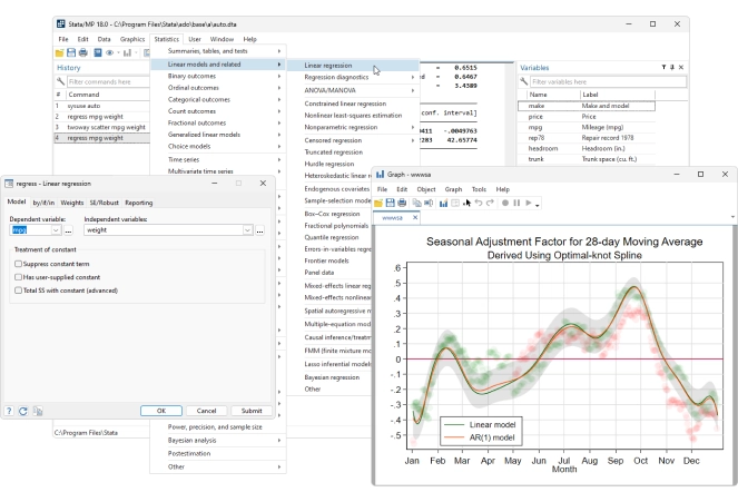
Publication Quality Graphics
Stata makes it easy to generate publication-quality, distinctly styled graphs.
You can point and click to create a custom graph. Or you can write scripts to produce hundreds or thousands of graphs in a reproducible manner.
Export graphs to EPS or TIFF for publication, to PNG or SVG for the web, or to PDF for viewing.
With the integrated Graph Editor, you click to change anything about your graph or to add titles, notes, lines, arrows, and text.
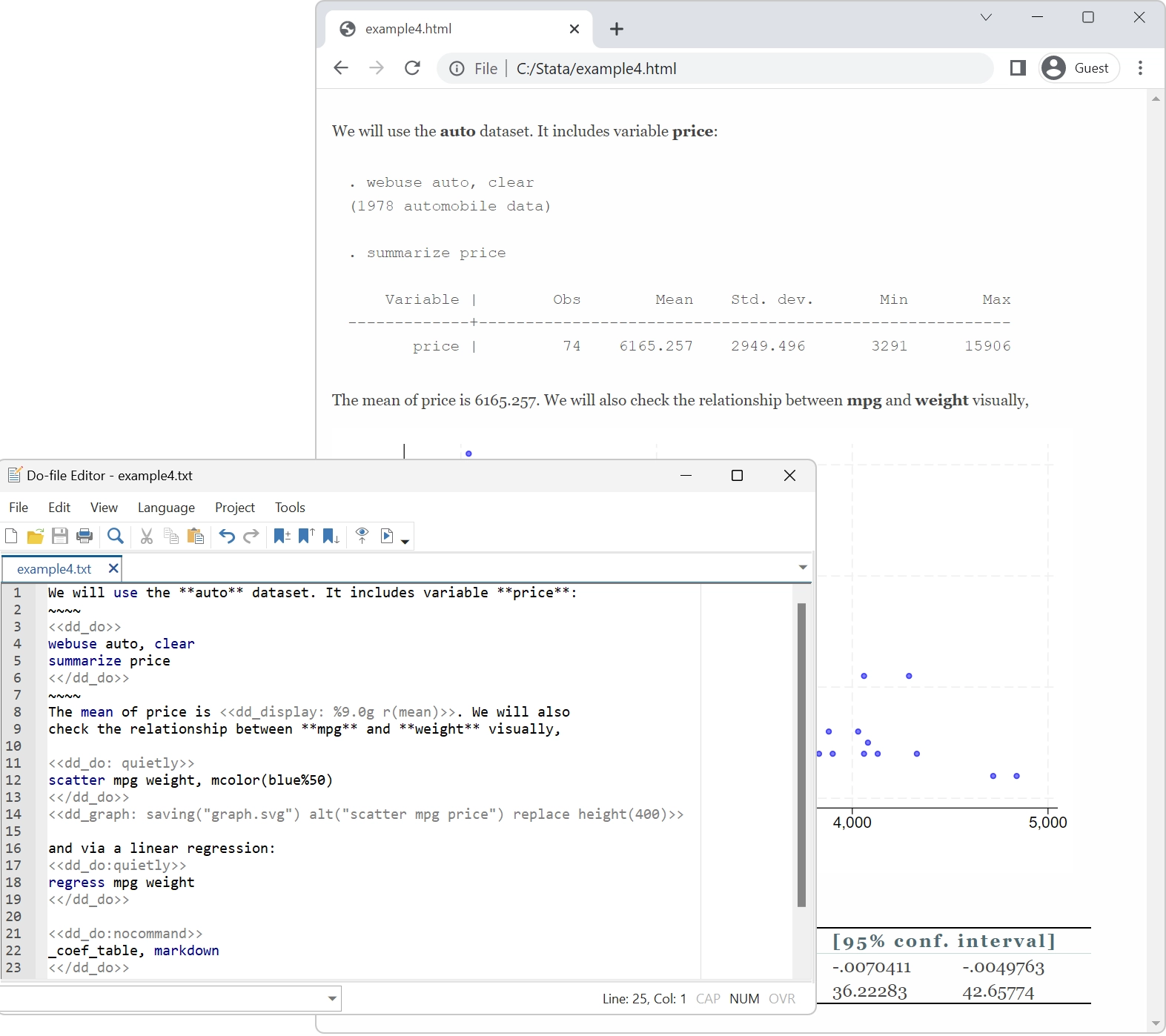
Automated Reporting
All the tools you need to automate reporting your results.
- Dynamic Markdown document
- Create Word documents
- Create PDF documents
- Create Excel files
- Customizable tables
- Schemes for graphics
- Word, HTML, PDF, SVG, PNG
Truly Reproducible Research
Many People talk about reproducible research. Stata has been dedicated to it for over 40 years.
We constantly add new features; we have even fundamentally changed language elements. No matter. Stata is the only statistical package with integrated versioning. If you wrote a script to perform an analysis in 1985, that same script will still run and still produce the same results today. Any dataset you created in 1985, you can read today. And the same will be true in 2050. Stata will be able to run anything you do today.
We take reproducibility seriously.
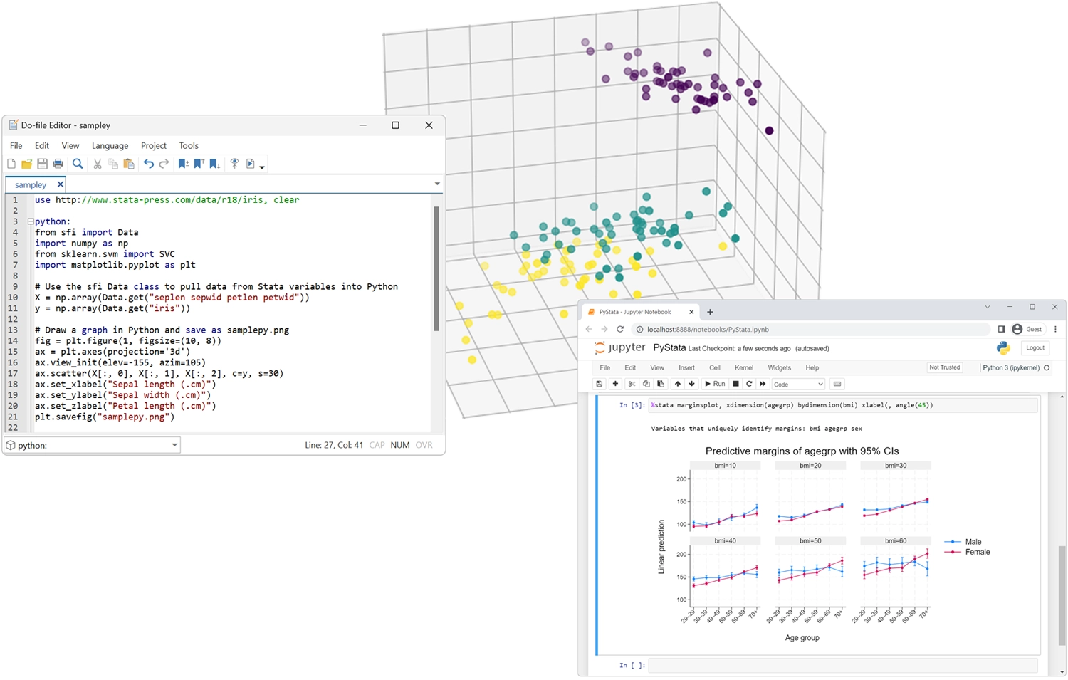
PyStata - Python Integration
Invoke Python interactively or embed Python in your Stata code.
Invoke Stata from Python and call Stata code from IPython environments.
Use Stata within Jupyter Notebook.
Seamlessly pass data and results between Stata and Python.
Use Stata analyses from within Python.
Use any Python package within Stata
- Matplotlib and seaborn for visualization
- Beautiful Soup and Scrapy for web scraping
- NumPy and pandas for numerical analysis
- TensorFlow and scikit-learn for machine learning
- And much more
Real Documentation
When it comes time to perform your analyses or understand the methods you are using, Stata does not leave you high and dry or ordering books to learn every detail.
Each of our data management features is fully explained and documented and shown in practice on real examples. Each estimator is fully documented and includes several examples on real data, with real discussions of how to interpret the results. The examples give you the data so you can work along in Stata and even extend the analyses. We give you a Quick start for every feature, showing some of the most common uses. Want even more detail? Our Methods and formulas sections provide the specifics of what is being computed, and our References point you to even more information.
Stata is a big package and so has lots of documentation – over 19,000 pages in 36 manuals. But don't worry, type help my topic, and Stata will search its keywords, indexes, and even community-contributed packages to bring you everything you need to know about your topic. Everything is available right within Stata.
Trusted
We don't just program statistical methods, we validate them.
The results you see from a Stata estimator rest on comparisons with other estimators, Monte Carlo simulations of consistency and coverage, and extensive testing by our statisticians. Every Stata we ship has passed a certification suite that includes 7.2 million lines of testing code that produces 6 million lines of output. We certify every number and piece of text from those 5.8 million lines of output.
Reliable
For over 40 years, StataCorp has been loyal to its users by expanding the Stata software with new statistical methods and the latest in reporting, data visualization, data manipulation, and the user interface. With our long-standing release history, we are committed to continually providing stable and reliable software to our diverse community of researchers and practitioners.
![]()
Continuously Updated
Staying on the most up-to-date version of Stata is now easier than ever.
StataCorp continually develops new features to enhance Stata software, from the latest statistical methods to the best in reporting, data visualization, and user interface. With StataNow™, new features are released throughout the current release until the next major release. These features are prioritized in the development cycle to be available as soon as they are ready so that users can take advantage of them right away.
![]()
Easy to Use
Staying on the most up-to-date version of Stata is now easier than ever.
All of Stata's features can be accessed through menus, dialogs, control panels, a Data Editor, a Variables Manager, a Graph Editor, and even an SEM Diagram Builder. You can point and click your way through any analysis.
If you don't want to write commands and scripts, you don't have to.
Even when you are pointing and clicking, you can record all your results and later include them in reports. You can even save the commands created by your actions and reproduce your complete analysis later.
Easy to Grow with
Stata's commands for performing tasks are intuitive and easy to learn. Even better, everything you learn about performing a task can be applied to other tasks. For example, you simply add if gender=="female" to any command to limit your analysis to females in your sample. You simply add vce(robust) to any estimator to obtain standard errors and hypothesis tests that are robust to many common assumptions.
The consistency goes even deeper. What you learn about data management commands often applies to estimation commands, and vice-versa. There is also a full suite of postestimation commands to perform hypothesis tests, form linear and nonlinear combinations, make predictions, form contrasts, and even perform marginal analysis with interaction plots. These commands work the same way after virtually every estimator.
Sequencing commands to read and clean data, then to perform statistical tests and estimation, and finally to report results is at the heart of reproducible research. Stata makes this process accessible to all researchers.
![]()
Easy to Automate
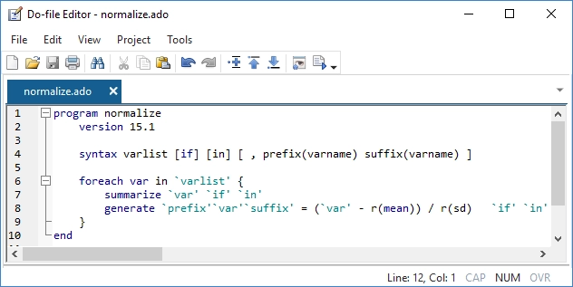
Everyone has tasks that they do all the time—create a particular kind of variable, produce a particular table, perform a sequence of statistical steps, compute an RMSE, etc. The possibilities are endless. Stata has thousands of built-in procedures, but you may have tasks that are relatively unique or that you want done in a specific way.
If you have written a script to perform your task on a given dataset, it is easy to transform that script into something that can be used on all your datasets, on any set of variables, and on any set of observations.
![]()
Easy to extend
Some of the things you automate may be so useful that you want to share them with colleagues or even make them available to all Stata users. That's also easy. With just a little code, you can turn an automation script into a Stata command. A command that supports standard features that Stata's official commands support. A command that can be used in the same way official commands are used.
Advanced Programming
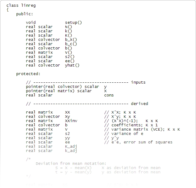
Stata also includes an advanced programming language—Mata.
Mata has the structures, pointers, and classes that you expect in your programming language and adds direct support for matrix programming.
Though you don't need to program to use Stata, it is comforting to know that a fast and complete programming language is an integral part of Stata. Mata is both an interactive environment for manipulating matrices and a full development environment that can produce compiled and optimized code. It includes special features for processing panel data, performs operations on real or complex matrices, provides complete support for object-oriented programming, and is fully integrated with every aspect of Stata. Stata also has comprehensive Python integration, allowing you to harness all the power of Python directly from your Stata code.
Stata also has PyStata, which provides comprehensive Python integration, allowing you to harness all the power of Python directly from your Stata code and to harness all the power of Stata from your Python code.
Stata even let's you incorporate C, C++, and Java plugins in your Stata programs via a native API for each language. And you can even embed Java code directly in your Stata code!

Community-contributed features
Stata is so programmable that developers and users add new features every day to respond to the growing demands of today's researchers.
With Stata's Internet capabilities, new features and official updates can be installed over the Internet with a single click.
World-class technical support
All registered users of the current release of Stata (Stata 19) are eligible for free technical support. If you have not registered your copy of Stata, please fill out the online registration form.
We have a dedicated staff of expert Stata programmers and statisticians to answer your technical questions. From tricky data management solutions to getting your graph looking just right and from explaining a robust standard error to specifying your multilevel model, we have your answers.
![]()
Cross-platform compatible
Stata will run on Windows, Mac, and Linux/Unix computers; however, our licenses are not platform specific. That means if you have a Mac laptop and a Windows desktop, you don't need two separate licenses to run Stata. You can install your Stata license on any of the supported platforms. Stata datasets, programs, and other data can be shared across platforms without translation. You can also quickly and easily import datasets from other statistical packages, spreadsheets, and databases.
Widely used
Used by researchers for more than 40 years, Stata provides everything you need for data science—data manipulation, visualization, statistics, and automated reporting.
Select your discipline and see how Stata can work for you.
Features For Data Scientists
Data wrangling
Scrape data from the web, import it from standard formats, or pull it in via SQL with JDBC or ODBC. Match-merge, link, append, reshape, transpose, sort, filter. Stata handles Unicode, frames (multiple datasets in memory), BLOBs, regular expressions, and more, whether working with hundreds of thousands or even billions of data points.
Automated reporting and customizable tables
Use Markdown to create Word documents and HTML files with embedded Stata code, output, and graphs. Automate Word, PDF, or Excel reports with both high-level export capabilities and low-level fine-grained programmatic access to automate production of the documents your team needs. Customize tables to clearly communicate results, and export your tables to Word, PDF, HTML, LaTeX, Excel, or Markdown.
Visualisation
Create graphs and customize them programmatically or interactively with the Graph Editor. Edits can even be recorded and "replayed" on other graphs for reproducibility. Export to industry standard formats suitable for web (SVG, PNG) or print (PDF, TIFF, EPS, PS).
Programming
Automate your entire workflow with both scripts and full-blown programming features like classes, structures, and pointers. A unique feature of Stata's programming environment is Mata, a fast and compiled matrix programming language. Of course, it has all the advanced matrix operations you need. It also has access to the power of LAPACK. What's more, it has built-in solvers and optimizers to make implementing your own estimator easier. And you can leverage all of Stata's estimation features and other features from within Mata.
PyStata—Python integration
Interact Stata code with Python code. You can seamlessly pass data and results between Stata and Python. You can use Stata within Jupyter Notebook and other IPython environments. You can call Python libraries such as NumPy, matplotlib, Scrapy, scikit-learn, and more from Stata. You can use Stata analyses from within Python.
Interoperability
Connect to external code via Python, Java, and C++ plugins. Write Python or Java code directly within your Stata code. Control Stata via Jupyter Notebook, OLE Automation, or call it in batch mode. Write custom SQL statements with JDBC and ODBC to extract from or populate databases. Access H2O clusters.
Statistics and modeling
Incorporate state-of-the-art statistical models and results in your workflow. Find groups in your data using unsupervised techniques including cluster analysis, principal components, factor analysis, multidimensional scaling, and correspondence analysis. Understand your groups even better using latent class analysis. When your analysis calls for supervised techniques, Stata has flexible nonparametric methods and an array of regression models from linear and logistic models to mixture models. Stata keeps up when your data call for special techniques. You have access to methods that understand and take advantage of the structure in time series, panel data, survival data, complex survey data, spatial data, and multilevel data. Stata provides the most approachable implementations of Bayesian methods and structural equation modeling available anywhere. You can request bootstrap methods for virtually any estimator. When your analysis calls for it, Stata automates other replication methods and simulations.
Reproducibility
Stata is the only software for data science and statistical analysis featuring a comprehensive version control system that ensures your code continues to run, unaltered, even after updates or new versions are released. No need to keep around multiple legacy installations to avoid breaking your system; Stata code from 25 years ago can still be run without modification. Datasets, graphs, scripts, programs, and more are 100% cross-platform and backward compatible.
Lasso
Use lasso and elastic net for model selection and prediction. And when you want to estimate effects and test coefficients for a few variables of interest, inferential methods provide estimates for these variables while using lassos to select from among a potentially large number of control variables. You can even account for endogenous covariates. Whether your goal is model selection, prediction, or inference, you can use Stata's lasso features with your continuous, binary, count, or time-to-event outcomes.
Features for Economists
Panel data
Take full advantage of the extra information that panel data provide while simultaneously handling the peculiarities of panel data. Study the time-invariant features within each panel, the relationships across panels, and how outcomes of interest change over time. Fit linear models or nonlinear models for binary, count, ordinal, censored, or survival outcomes with fixed-effects, random-effects, or population-averaged estimators. Fit dynamic models or models with endogeneity.
Time series
Handle the statistical challenges inherent to time-series data—autocorrelations, common factors, autoregressive conditional heteroskedasticity, unit roots, cointegration, and much more. Analyze univariate time series using ARIMA, ARFIMA, Markov-switching models, ARCH and GARCH models, and unobserved-components models. Compare ARIMA or ARFIMA models using AIC, BIC, and HQIC, and select the best number of autoregressive and moving-average terms. Analyze multivariate time series using VAR, structural VAR, VEC, multivariate GARCH, dynamic-factor models, and state-space models. Compute and graph impulse responses. Test for unit roots. Perform Bayesian time-series analysis.
Cross-sectional models
Fit classical linear models of the relationship between a continuous outcome, such as wage, and the determinants of wage, such as education level, age, experience, and economic sector. If your response is binary (for example, employed or unemployed), ordinal (education level), count (number of children), or censored (ticket sales in an existing venue), don't worry. Stata has maximum likelihood estimators—probit, ordered probit, Poisson, tobit, and many others—that estimate the relationship between such outcomes and their determinants. A vast array of tools is available to analyze such models. Predict outcomes and their confidence intervals. Test equality of parameters, or any linear or nonlinear combination of parameters.
Endogeneity and selection
When explanatory variables are related to omitted observable variables, or when they are related to unobservable variables, or when there is selection bias, then causal relationships are confounded and parameter estimates from standard estimators produce inconsistent estimates of the true relationships. Stata can fit consistent models when there is such endogeneity or selection—whether your outcome variable is continuous, binary, count, or ordinal and whether your data are cross-sectional or panel. Stata can even combine endogenous covariates, selection, and treatment effects in the same model.
Causal inference/Treatment effects
Estimate experimental-style causal effects from observational data; for instance, estimate the effect of a job training program on employment or the effect of a subsidy on production. Fit models for continuous, binary, count, fractional, and survival outcomes with binary or multivalued treatments using inverse-probability weighting (IPW), propensity-score matching, nearest-neighbor matching, regression adjustment, or doubly robust estimators. Fit models with exogenous or endogenous treatments. After estimation, test the overlap assumption and covariate balance. Add endogenous covariates and sample selection to some treatment-effects estimators. In the presence of group and time effects, you can use difference-in-differences (DID) and triple-differences (DDD) estimators. In the presence of high-dimensional covariates, you can use lasso. If causal effects are mediated through another variable, use causal mediation with mediate to disentangle direct and indirect effects.
Marginal effects and marginal means
Marginal effects and marginal means let you analyze and visualize the relationships between your outcome variable and your covariates, even when that outcome is binary, count, ordinal, categorical, or censored (tobit). Estimate population-averaged marginal effects or evaluate marginal effects at interesting or representative values of the covariates. Analyze the effect of interactions. You can even trace out the marginal effect over a range of interesting covariate values or covariate interactions. You can do all of this with marginal means (sometimes called potential-outcome means), even when your “mean” is a probability of a positive outcome or a count from a Poisson model. If you have panel data and random effects, these effects are automatically integrated out to provide marginal (that is, population-averaged) effects.
Choice models
Model your discrete choice data. If your outcome is, for instance, a choice to travel by bus, train, car, or airplane, you can fit a conditional logit, multinomial probit, or mixed logit model. Is your outcome instead a ranking of prefered travel methods? Fit a rank-ordered probit or rank-ordered logit model. Regardless of the model fit, you can use the margins to easily interpret the results. Estimate how much wait times at the airport affect the probability of traveling by air or even by train.
GMM
GMM (generalized method of moments) can be used to fit almost any statistical model, including both exactly identified and overidentified estimation problems. Overidentified problems arise when you have endogeneity, correlation in dynamic panels, sample selection, and many other situations. With Stata, you estimate these models by simply writing your moments and enclosing the parameters in curly braces. You can easily fit cross-sectional, time-series, panel-data, or survival-data models and test your overidentifying restrictions.
Demand systems
Fit demand systems to explore consumers' demand for goods and services. Given a budget and a bundle of goods and services, determine the expenditure and price elasticities for these goods. Choose between the Cobb–Douglas system, Stone's linear expenditure system, the translog indirect utility demand system, the almost ideal demand system (AIDS), the quadratic almost ideal demand system (QUAIDS), and others.
Lasso
Use lasso and elastic net for model selection and prediction. And when you want to estimate effects and test coefficients for a few variables of interest, inferential methods provide estimates for these variables while using lassos to select from among a potentially large number of control variables. You can even account for endogenous covariates. Whether your goal is model selection, prediction, or inference, you can use Stata's lasso features with your continuous, binary, count, or time-to-event outcomes.
Programming
Want to program your own commands to perform estimation, perform data management, or implement other new features? Stata is programmable, and thousands of Stata users have implemented and published thousands of community-contributed commands. These commands look and act just like official Stata commands and are easily installed for free over the Internet from within Stata. A unique feature of Stata's programming environment is Mata, a fast and compiled language with support for matrix types. Of course, it has all the advanced matrix operations you need. It also has access to the power of LAPACK. What's more, it has built-in solvers and optimizers to make implementing your own maximum likelihood, GMM, or other estimators easier. And you can leverage all of Stata's estimation and other features from within Mata. Many of Stata's official commands are themselves implemented in Mata.
PyStata - Python integration
Interact Stata code with Python code. You can seamlessly pass data and results between Stata and Python. You can use Stata within Jupyter Notebook and other IPython environments. You can call Python libraries such as NumPy, matplotlib, Scrapy, scikit-learn, and more from Stata. You can use Stata analyses from within Python.
Forecasting
Build multiequation models, and produce forecasts of levels, trends, rates, etc. Whether you have a small model with a few equations or a complete model of the economy with thousands of equations, Stata can help you build that model and produce forecasts. Your model can include both estimated relationships and known identities. You can easily create and compare forecasts under different scenarios, create static and dynamic forecasts, and even estimate stochastic confidence intervals. You can create your model by using an intuitive command syntax or by using the interactive forecasting control panel.
Survival Analysis
Analyze duration outcomes—outcomes measuring the time to an event such as failure or death—using Stata's specialized tools for survival analysis. Account for the complications inherent in survival data, such as sometimes not observing the event (right-, left-, and interval-censoring), individuals entering the study at differing times (delayed entry), and individuals who are not continuously observed throughout the study (gaps). You can estimate and plot the probability of survival over time. Or model survival as a function of covariates using Cox, Weibull, lognormal, and other regression models. Predict hazard ratios, mean survival time, and survival probabilities. Do you have groups of individuals in your study? Adjust for within-group correlation with a random-effects or shared-frailty model. If you have many potential covariates, use lasso cox and elasticnet cox for model selection and prediction.
Bayesian analysis
Perform Bayesian econometrics analysis using one of the Markov chain Monte Carlo (MCMC) methods. You can choose from various supported models, such as panel-data, hierarchical, VAR, and DSGE models, or you can even program your own. Extensive tools are available to check convergence, including multiple chains. Compute posterior mean estimates and credible intervals for model parameters and functions of model parameters. You can perform both interval- and model-based hypothesis testing. Compare models using Bayes factors. Compute model fit using posterior predictive values. Generate predictions and forecasts. If you want to account for model uncertainty in your regression model, use Bayesian model averaging.
Survey methods
Whether your data require a simple weighted adjustment because of differential sampling rates or you have data from a complex multistage survey, Stata's survey features can provide you with correct standard errors and confidence intervals for your inferences. Simply specify the relevant characteristics of your sampling design, such as sampling weights (including weights at multiple stages), clustering (at one, two, or more stages), stratification, and poststratification. After that, most of Stata's estimation commands can adjust their estimates to correct for your sampling design.
Meta-analysis
Combine results of multiple studies to estimate an overall effect. Use forest plots to visualize results. Use subgroup analysis and meta-regression to explore study heterogeneity. Use funnel plots and formal tests to explore publication bias and small-study effects. Use trim-and-fill analysis to assess the impact of publication bias on results. Perform cumulative and leave-one-out meta-analysis. Perform univariate, multilevel, and multivariate meta-analysis. Use the meta suite, or let the Control Panel interface guide you through your entire meta-analysis.
Automated reporting and customizable tables
Stata is designed for reproducible research, including the ability to create dynamic documents incorporating your analysis results. Create Word or PDF files, populate Excel worksheets with results and format them to your liking, and mix Markdown, HTML, Stata results, and Stata graphs, all from within Stata. Create tables that compare regression results or summary statistics, use default styles or apply your own, and export your tables to Word, PDF, HTML, LaTeX, Excel, or Markdown and include them in your reports.
Features for Education
Multilevel mixed-effects models
Whether the groupings in your data arise in a nested fashion (students nested in classrooms and classrooms nested in schools) or in a nonnested fashion (elementary school crossed with middle school), you can fit a multilevel model to account for the lack of independence within these groups. Fit models for continuous, binary, count, ordinal, and survival outcomes. Estimate variances of random intercepts and random coefficients. Compute intraclass correlations. Predict random effects. Estimate relationships that are population averaged over the random effects.
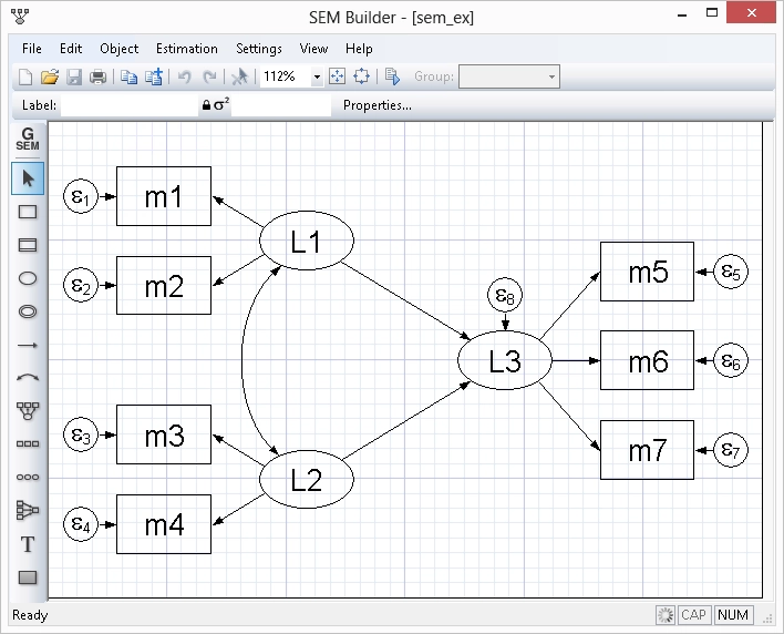
Structural equation modeling (SEM)
Estimate mediation effects, analyze the relationship between an unobserved latent concept such as verbal abilities and the observed variables that measure verbal abilities, or fit a model with complex relationships among both latent and observed variables. Fit models with continuous, binary, count, and ordinal outcomes. Even fit hierarchical models with groups of correlated observations such as children within the same schools. Evaluate model fit. Compute indirect and total effects. Fit models by drawing a path diagram or using the straightforward command syntax.
General Linear Models
Fit one- and two-way models. Or fit models with three, four, or even more factors. Analyze data with nested factors, with fixed and random factors, or with repeated measures. Use ANCOVA models when you have continuous covariates and MANOVA models when you have multiple outcome variables. Further explore the relationships between your outcome and predictors by estimating effect sizes and computing least-squares and marginal means. Perform contrasts and pairwise comparisons. Analyze and plot interactions.
IRT (item response theory)
Explore the relationship between unobserved latent characteristics such as mathematical aptitude and the probability of correctly answering test questions (items). Or explore the relationship between teacher job satisfaction and self-reported responses to questions related to job statisfaction. IRT can be used to create measures of such unobserved traits or place individuals on a scale measuring the trait. It can also be used to select the best items for measuring a latent trait. IRT models are available for binary, graded, rated, partial-credit, and nominal response items. Visualize the relationships using item characteristic curves, and measure overall test performance using test information functions.
Linear, binary and count regressions
Fit classical linear regression models of the relationship between a continuous outcome, such as a reading test score, and the determinants of the score, such as teaching method and the student's reading level in the previous grade. If your response is binary (for example, pass or fail test), ordinal (education level), count (number of students), or categorical (private, public, or home school), don't worry. Stata has maximum likelihood estimators—logistic, ordered logistic, Poisson, multinomial logit, and many others—that estimate the relationship between such outcomes and their determinants. A vast array of tools is available after fitting such models. Predict outcomes and their confidence intervals. Test equality of parameters. Compute linear and nonlinear combinations of parameters.
Linear, binary and count regressions
Account for missing data in your sample using multiple imputation. Choose from univariate and multivariate methods to impute missing values in continuous, censored, truncated, binary, ordinal, categorical, and count variables. Then, in a single step, estimate parameters using the imputed datasets, and combine results. Fit a linear model, logit model, Poisson model, hierarchical model, survival model, or one of the many other supported models. Use the mi command, or let the Control Panel interface guide you through your entire MI analysis.
Choice models
Model your discrete choice data. If your outcome is, for instance, a choice to travel by bus, train, car, or airplane, you can fit a conditional logit, multinomial probit, or mixed logit model. Is your outcome instead a ranking of prefered travel methods? Fit a rank-ordered probit or rank-ordered logit model. Regardless of the model fit, you can use the margins to easily interpret the results. Estimate how much wait times at the airport affect the probability of traveling by air or even by train.
Contrasts, marginal means and profile plots
Quickly and easily obtain contrasts for categorical variables and their interactions. R.edlevel will give you all the contrasts of education level with a reference category. A.edlevel will give you each paired contrast with the next higher education level. There are many more named contrasts, and you can specify your own. If you don't like typing, use a dialog box to select your contrasts. Marginal means are just a simple command or mouse click away after almost any estimation command. Evaluating interaction effects, the effects of moderating variables, is just as easy. And this is not just for linear models, but for models with binary, ordinal, and count outcomes. Even for hierarchical models with correct handling of random effects. A simple command or a few mouse clicks will get you a profile plot of any of these results.
Power, precision and sample size
Before you conduct your experiment, determine the sample size needed to detect meaningful effects without wasting resources. Do you intend to compute CIs for means or variances or perform tests for proportions or correlations? Do you plan to fit a Cox proportional hazards model or compare survivor functions using a log-rank test? Do you want to use a Cochran—Mantel—Haenszel test of association or a Cochran—Armitage trend test? Use Stata's power command to compute power and sample size, create customized tables, and automatically graph the relationships between power, sample size, and effect size for your planned study. Or use the ciwidth command to do the same but for CIs instead of hypothesis tests by computing the required sample size for the desired CI precision. Or use gsdesign to compute stopping boundaries and the required sample sizes for group sequential designs. Instead of commands, use the interactive Control Panel to perform your analysis.
Causal Inference
Estimate experimental-style causal effects from observational data. With Stata's treatment-effects estimators, you can use a potential-outcomes (counterfactuals) framework to estimate, for instance, the effect of family structure on child development or the effect of unemployment on anxiety. Fit models for continuous, binary, count, fractional, and survival outcomes with binary or multivalued treatments using inverse-probability weighting (IPW), propensity-score matching, nearest-neighbor matching, regression adjustment, or doubly robust estimators. If the assignment to a treatment is not independent of the outcome, you can use an endogenous treatment-effects estimator. In the presence of group and time effects, you can use difference-in-differences (DID) and triple-differences (DDD) estimators. In the presence of high-dimensional covariates, you can use lasso. If causal effects are mediated through another variable, use causal mediation with mediate to disentangle direct and indirect effects.
Multivariate methods
Use multivariate analyses to evaluate relationships among variables from many different perspectives. Perform multivariate tests of means, or fit multivariate regression and MANOVA models. Explore relationships between two sets of variables, such as aptitude measurements and achievement measurements, using canonical correlation. Examine the number and structure of latent concepts underlying a set of variables using exploratory factor analysis. Or use principal component analysis to find underlying structure or to reduce the number of variables used in a subsequent analysis. Discover groupings of observations in your data using cluster analysis. If you have known groups in your data, describe differences between them using discriminant analysis.
Automated reporting and customizable tables
Stata is designed for reproducible research, including the ability to create dynamic documents incorporating your analysis results. Create Word or PDF files, populate Excel worksheets with results and format them to your liking, and mix Markdown, HTML, Stata results, and Stata graphs, all from within Stata. Create tables that compare regression results or summary statistics, use default styles or apply your own, and export your tables to Word, PDF, HTML, LaTeX, Excel, or Markdown and include them in your reports.
Bayesian analysis
Perform Bayesian econometrics analysis using one of the Markov chain Monte Carlo (MCMC) methods. You can choose from various supported models, such as panel-data, hierarchical, VAR, and DSGE models, or you can even program your own. Extensive tools are available to check convergence, including multiple chains. Compute posterior mean estimates and credible intervals for model parameters and functions of model parameters. You can perform both interval- and model-based hypothesis testing. Compare models using Bayes factors. Compute model fit using posterior predictive values. Generate predictions and forecasts. If you want to account for model uncertainty in your regression model, use Bayesian model averaging.
Meta-analysis
Combine results of multiple studies to estimate an overall effect. Use forest plots to visualize results. Use subgroup analysis and meta-regression to explore study heterogeneity. Use funnel plots and formal tests to explore publication bias and small-study effects. Use trim-and-fill analysis to assess the impact of publication bias on results. Perform cumulative and leave-one-out meta-analysis. Perform univariate, multilevel, and multivariate meta-analysis. Use the meta suite, or let the Control Panel interface guide you through your entire meta-analysis.
Jupyter Notebook with Stata
Jupyter Notebook is widely used by researchers and scientists to share their ideas and results for collaboration and innovation. It is an easy-to-use web application that allows you to combine code, visualizations, mathematical formulas, narrative text, and other rich media in a single document (a "notebook") for interactive computing and developing. You can invoke Stata and Mata from Jupyter Notebook with the IPython (interactive Python) kernel. This means you can combine the capabilities of both Python and Stata in a single environment to make your work easily reproducible and shareable with others.
Features for Epidemiologists
Epidemiological tables
Want to analyze data from a prospectiv321 laddence") study, cohort study, case–control study, or matched case–control study? Stata's tables for epidemiologists make it easy to summarize your data and compute statistics such as incidence-rate ratios, incidence-rate differences, risk ratios, risk differences, odds ratios, and attributable fractions. You can analyze stratified data too—compute Mantel–Haenszel combined estimates, perform tests of homogeneity, and standardize estimates. If you have an ordinal rather than binary exposure, you can perform a test for a trend.
Survival analysis
Analyze duration outcomes—outcomes measuring the time to an event such as failure or death—using Stata's specialized tools for survival analysis. Account for the complications inherent in survival data, such as sometimes not observing the event (right-, left-, and interval-censoring), individuals entering the study at differing times (delayed entry), and individuals who are not continuously observed throughout the study (gaps). You can estimate and plot the probability of survival over time. Or model survival as a function of covariates using Cox, Weibull, lognormal, and other regression models. Predict hazard ratios, mean survival time, and survival probabilities. Do you have groups of individuals in your study? Adjust for within-group correlation with a random-effects or shared-frailty model. If you have many potential covariates, use lasso cox and elasticnet cox for model selection and prediction.
Linear, binary and count regressions
Fit classical ANOVA and linear regression models of the relationship between a continuous outcome, such as weight, and the determinants of weight, such as height, diet, and level of exercise. If your response is binary, ordinal, categorical, or count, don't worry. Stata has estimators for these types of outcomes too. Use logistic regression to adjust odds ratios for confounding variables. Estimate incidence rates using a Poisson model. Analyze matched case–control data with conditional logistic regression. A vast array of tools is available after fitting such models. Predict outcomes and their confidence intervals. Test equality of parameters. Compute linear and nonlinear combinations of parameters.
Survey methods
Whether your data require a simple weighted adjustment because of differential sampling rates or you have data from a complex multistage survey, Stata's survey features can provide you with correct standard errors and confidence intervals for your inferences. Simply specify the relevant characteristics of your sampling design, such as sampling weights (including weights at multiple stages), clustering (at one, two, or more stages), stratification, and poststratification. After that, most of Stata's estimation commands can adjust their estimates to correct for your sampling design.
Marginal means, contrasts and interactions
Marginal means and contrasts let you analyze the relationships between your outcome variable and your predictors, even when your outcome is binary, count, ordinal, or categorical. For instance, after you fit a logistic regression of a disease on an exposure variable and other covariates, your marginal means may be population-averaged risks. Or you can set the covariates to interesting values to compute adjusted risks and then use contrasts to get adjusted risk differences. After fitting almost any model in Stata, you can analyze the effect of covariate interactions and easily create plots to visualize those interactions.
Power, precision and sample size
Before you conduct your experiment, determine the sample size needed to detect meaningful effects without wasting resources. Do you intend to compute CIs for means or variances or perform tests for proportions or correlations? Do you plan to fit a Cox proportional hazards model or compare survivor functions using a log-rank test? Do you want to use a Cochran—Mantel—Haenszel test of association or a Cochran—Armitage trend test? Use Stata's power command to compute power and sample size, create customized tables, and automatically graph the relationships between power, sample size, and effect size for your planned study. Or use the ciwidth command to do the same but for CIs instead of hypothesis tests by computing the required sample size for the desired CI precision. Or use gsdesign to compute stopping boundaries and the required sample sizes for group sequential designs. Instead of commands, use the interactive Control Panel to perform your analysis.
Meta-analysis
Combine results of multiple studies to estimate an overall effect. Use forest plots to visualize results. Use subgroup analysis and meta-regression to explore study heterogeneity. Use funnel plots and formal tests to explore publication bias and small-study effects. Use trim-and-fill analysis to assess the impact of publication bias on results. Perform cumulative and leave-one-out meta-analysis. Perform univariate, multilevel, and multivariate meta-analysis. Use the meta suite, or let the Control Panel interface guide you through your entire meta-analysis.
Causal inference
Estimate experimental-style causal effects from observational data. With Stata's treatment-effects estimators, you can use a potential-outcomes (counterfactuals) framework to estimate, for instance, the effect of family structure on child development or the effect of unemployment on anxiety. Fit models for continuous, binary, count, fractional, and survival outcomes with binary or multivalued treatments using inverse-probability weighting (IPW), propensity-score matching, nearest-neighbor matching, regression adjustment, or doubly robust estimators. If the assignment to a treatment is not independent of the outcome, you can use an endogenous treatment-effects estimator. In the presence of group and time effects, you can use difference-in-differences (DID) and triple-differences (DDD) estimators. In the presence of high-dimensional covariates, you can use lasso. If causal effects are mediated through another variable, use causal mediation with mediate to disentangle direct and indirect effects.
Multiple imputation
Account for missing data in your sample using multiple imputation. Choose from univariate and multivariate methods to impute missing values in continuous, censored, truncated, binary, ordinal, categorical, and count variables. Then, in a single step, estimate parameters using the imputed datasets, and combine results. Fit a linear model, logit model, Poisson model, multilevel model, survival model, or one of the many other supported models. Use the mi command, or let the Control Panel interface guide you through your entire MI analysis.
Multilevel mixed-effects models
Whether the groupings in your data arise in a nested fashion (patients nested in clinics and clinics nested in regions) or in a nonnested fashion (regions crossed with occupations), you can fit a multilevel model to account for the lack of independence within these groups. Fit models for continuous, binary, count, ordinal, and survival outcomes. Estimate variances of random intercepts and random coefficients. Compute intraclass correlations. Predict random effects. Estimate relationships that are population averaged over the random effects.
Bayesian analysis
Fit Bayesian regression models using one of the Markov chain Monte Carlo (MCMC) methods. You can choose from various supported models or even program your own. Extensive tools are available to check convergence, including multiple chains. Compute posterior mean estimates and credible intervals for model parameters and functions of model parameters. You can perform both interval- and model-based hypothesis testing. Compare models using Bayes factors. Compute model fit using posterior predictive values and generate predictions. If you want to account for model uncertainty in your regression model, use Bayesian model averaging.
Additive models of relative risk
Determine how exposures interact to put subjects at a higher risk of experiencing an outcome of interest. For example, you might be investigating how exposure to cigarette smoke and asbestos interact to increase the risk of lung cancer. With Stata's reri command, you can measure two–way interactions in an additive model of relative risk, while accounting for other risk factors. Choose from various supported models, such as binomial generalized linear, Poisson, negative binomial, logistic, Cox, parametric survival, and interval–censored parametric and semiparametric survival models. Estimate the relative excess risk due to interaction (RERI), attributable proportion (AP), and synergy index (SI).
Automated reporting and customizable tables
Stata is designed for reproducible research, including the ability to create dynamic documents incorporating your analysis results. Create Word or PDF files, populate Excel worksheets with results and format them to your liking, and mix Markdown, HTML, Stata results, and Stata graphs, all from within Stata. Create tables that compare regression results or summary statistics, use default styles or apply your own, and export your tables to Word, PDF, HTML, LaTeX, Excel, or Markdown and include them in your reports.
Jupyter Notebook with Stata
Jupyter Notebook is widely used by researchers and scientists to share their ideas and results for collaboration and innovation. It is an easy-to-use web application that allows you to combine code, visualizations, mathematical formulas, narrative text, and other rich media in a single document (a "notebook") for interactive computing and developing. You can invoke Stata and Mata from Jupyter Notebook with the IPython (interactive Python) kernel. This means you can combine the capabilities of both Python and Stata in a single environment to make your work easily reproducible and shareable with others.
Features for Biostatisticians
Survival analysis
Analyze duration outcomes—outcomes measuring the time to an event such as failure or death—using Stata's specialized tools for survival analysis. Account for the complications inherent in survival data, such as sometimes not observing the event (right-, left-, and interval-censoring), individuals entering the study at differing times (delayed entry), and individuals who are not continuously observed throughout the study (gaps). You can estimate and plot the probability of survival over time. Or model survival as a function of covariates using Cox, Weibull, lognormal, and other regression models. Predict hazard ratios, mean survival time, and survival probabilities. Do you have groups of individuals in your study? Adjust for within-group correlation with a random-effects or shared-frailty model. If you have many potential covariates, use lasso cox and elasticnet cox for model selection and prediction.
Multilevel mixed-effects models
Whether the groupings in your data arise in a nested fashion (patients nested in clinics and clinics nested in regions) or in a nonnested fashion (regions crossed with occupations), you can fit a multilevel model to account for the lack of independence within these groups. Fit models for continuous, binary, count, ordinal, and survival outcomes. Estimate variances of random intercepts and random coefficients. Compute intraclass correlations. Predict random effects. Estimate relationships that are population averaged over the random effects.
Bayesian analysis
Fit Bayesian regression models using one of the Markov chain Monte Carlo (MCMC) methods. You can choose from various supported models or even program your own. Extensive tools are available to check convergence, including multiple chains. Compute posterior mean estimates and credible intervals for model parameters and functions of model parameters. You can perform both interval- and model-based hypothesis testing. Compare models using Bayes factors. Compute model fit using posterior predictive values and generate predictions. If you want to account for model uncertainty in your regression model, use Bayesian model averaging.
Power, precision and sample size
Before you conduct your experiment, determine the sample size needed to detect meaningful effects without wasting resources. Do you intend to compute CIs for means or variances or perform tests for proportions or correlations? Do you plan to fit a Cox proportional hazards model or compare survivor functions using a log-rank test? Do you want to use a Cochran—Mantel—Haenszel test of association or a Cochran—Armitage trend test? Use Stata's power command to compute power and sample size, create customized tables, and automatically graph the relationships between power, sample size, and effect size for your planned study. Or use the ciwidth command to do the same but for CIs instead of hypothesis tests by computing the required sample size for the desired CI precision. Or use gsdesign to compute stopping boundaries and the required sample sizes for group sequential designs. Instead of commands, use the interactive Control Panel to perform your analysis.
Linear, binary and count regressions
Fit classical ANOVA and linear regression models of the relationship between a continuous outcome, such as weight, and the determinants of weight, such as height, diet, and level of exercise. If your response is binary, ordinal, categorical, or count, don't worry. Stata has estimators for these types of outcomes too. Use logistic regression to estimate odds ratios. Estimate incidence rates using a Poisson model. Analyze matched case–control data with conditional logistic regression. A vast array of tools is available after fitting such models. Predict outcomes and their confidence intervals. Test equality of parameters. Compute linear and nonlinear combinations of parameters.
Meta-analysis
Combine results of multiple studies to estimate an overall effect. Use forest plots to visualize results. Use subgroup analysis and meta-regression to explore study heterogeneity. Use funnel plots and formal tests to explore publication bias and small-study effects. Use trim-and-fill analysis to assess the impact of publication bias on results. Perform cumulative and leave-one-out meta-analysis. Perform univariate, multilevel, and multivariate meta-analysis. Use the meta suite, or let the Control Panel interface guide you through your entire meta-analysis.
Multiple imputation
Account for missing data in your sample using multiple imputation. Choose from univariate and multivariate methods to impute missing values in continuous, censored, truncated, binary, ordinal, categorical, and count variables. Then, in a single step, estimate parameters using the imputed datasets, and combine results. Fit a linear model, logit model, Poisson model, hierarchical model, survival model, or one of the many other supported models. Use the mi command, or let the Control Panel interface guide you through your entire MI analysis.
Marginal means, contrasts and interactions
Marginal means and contrasts let you analyze the relationships between your outcome variable and your covariates, even when that outcome is binary, count, ordinal, categorical, or survival. Compute adjusted predictions with covariates set to interesting or representative values. Or compute marginal means for each level of a categorical covariate. Make comparisons of the adjusted predictions or marginal means using contrasts. If you have multilevel data and random effects, these effects are automatically integrated out to provide marginal (that is, population-averaged) estimates. After fitting almost any model in Stata, analyze the effect of covariate interactions, and easily create plots to visualize those interactions.
Causal inference
Estimate experimental-style causal effects from observational data. With Stata's treatment-effects estimators, you can use a potential-outcomes (counterfactuals) framework to estimate, for instance, the effect of family structure on child development or the effect of unemployment on anxiety. Fit models for continuous, binary, count, fractional, and survival outcomes with binary or multivalued treatments using inverse-probability weighting (IPW), propensity-score matching, nearest-neighbor matching, regression adjustment, or doubly robust estimators. If the assignment to a treatment is not independent of the outcome, you can use an endogenous treatment-effects estimator. In the presence of group and time effects, you can use difference-in-differences (DID) and triple-differences (DDD) estimators. In the presence of high-dimensional covariates, you can use lasso. If causal effects are mediated through another variable, use causal mediation with mediate to disentangle direct and indirect effects.
Epidemiological tables
Want to analyze data from a prospective (incidence) study, cohort study, case–control study, or matched case–control study? Stata's tables for epidemiologists make it easy to summarize your data and compute statistics such as incidence-rate ratios, incidence-rate differences, risk ratios, risk differences, odds ratios, and attributable fractions. You can analyze stratified data too—compute Mantel–Haenszel combined estimates, perform tests of homogeneity, and standardize estimates. If you have an ordinal rather than binary exposure, you can perform a test for a trend.
Programming
Want to program your own commands to perform estimation, perform data management, or implement other new features? Stata is programmable, and thousands of Stata users have implemented and published thousands of community-contributed commands. These commands look and act just like official Stata commands and are easily installed for free over the Internet from within Stata. A unique feature of Stata's programming environment is Mata, a fast and compiled language with support for matrix types. Of course, it has all the advanced matrix operations you need. It also has access to the power of LAPACK. What's more, it has built-in solvers and optimizers to make implementing your own maximum likelihood, GMM, or other estimators easier. And you can leverage all of Stata's estimation and other features from within Mata. Many of Stata's official commands are themselves implemented in Mata.
PyStata - Python integration
Interact Stata code with Python code. You can seamlessly pass data and results between Stata and Python. You can use Stata within Jupyter Notebook and other IPython environments. You can call Python libraries such as NumPy, matplotlib, Scrapy, scikit-learn, and more from Stata. You can use Stata analyses from within Python.
Automated reporting and customizable tables
Stata is designed for reproducible research, including the ability to create dynamic documents incorporating your analysis results. Create Word or PDF files, populate Excel worksheets with results and format them to your liking, and mix Markdown, HTML, Stata results, and Stata graphs, all from within Stata. Create tables that compare regression results or summary statistics, use default styles or apply your own, and export your tables to Word, PDF, HTML, LaTeX, Excel, or Markdown and include them in your reports.
Features for Medical Researchers
General linear models
Fit one- and two-way models. Or fit models with three, four, or even more factors. Analyze data with nested factors, with fixed and random factors, or with repeated measures. Use ANCOVA models when you have continuous covariates and MANOVA models when you have multiple outcome variables. Further explore the relationships between your outcome and predictors by estimating effect sizes and computing least-squares and marginal means. Perform contrasts and pairwise comparisons. Analyze and plot interactions.
Linear, binary and count regressions
Fit classical ANOVA and linear regression models of the relationship between a continuous outcome, such as weight, and the determinants of weight, such as height, diet, and level of exercise. If your response is binary, ordinal, categorical, or count, don't worry. Stata has estimators for these types of outcomes too. Use logistic regression to estimate odds ratios. Estimate incidence rates using a Poisson model. Analyze matched case–control data with conditional logistic regression. A vast array of tools is available after fitting such models. Predict outcomes and their confidence intervals. Test equality of parameters. Compute linear and nonlinear combinations of parameters.
Power, precision and sample size
Before you conduct your experiment, determine the sample size needed to detect meaningful effects without wasting resources. Do you intend to compute CIs for means or variances or perform tests for proportions or correlations? Do you plan to fit a Cox proportional hazards model or compare survivor functions using a log-rank test? Do you want to use a Cochran—Mantel—Haenszel test of association or a Cochran—Armitage trend test? Use Stata's power command to compute power and sample size, create customized tables, and automatically graph the relationships between power, sample size, and effect size for your planned study. Or use the ciwidth command to do the same but for CIs instead of hypothesis tests by computing the required sample size for the desired CI precision. Or use gsdesign to compute stopping boundaries and the required sample sizes for group sequential designs. Instead of commands, use the interactive Control Panel to perform your analysis.
Marginal means, contrasts and interactions
Marginal means and contrasts let you analyze the relationships between your outcome variable and your covariates, even when that outcome is binary, count, ordinal, categorical, or survival. Compute adjusted predictions with covariates set to interesting or representative values. Or compute marginal means for each level of a categorical covariate. Make comparisons of the adjusted predictions or marginal means using contrasts. If you have multilevel data and random effects, these effects are automatically integrated out to provide marginal (that is, population-averaged) estimates. After fitting almost any model in Stata, analyze the effect of covariate interactions, and easily create plots to visualize those interactions.
Multilevel mixed-effects models
Whether the groupings in your data arise in a nested fashion (patients nested in clinics and clinics nested in regions) or in a nonnested fashion (regions crossed with occupations), you can fit a multilevel model to account for the lack of independence within these groups. Fit models for continuous, binary, count, ordinal, and survival outcomes. Estimate variances of random intercepts and random coefficients. Compute intraclass correlations. Predict random effects. Estimate relationships that are population averaged over the random effects.
Meta-analysis
Combine results of multiple studies to estimate an overall effect. Use forest plots to visualize results. Use subgroup analysis and meta-regression to explore study heterogeneity. Use funnel plots and formal tests to explore publication bias and small-study effects. Use trim-and-fill analysis to assess the impact of publication bias on results. Perform cumulative and leave-one-out meta-analysis. Perform univariate, multilevel, and multivariate meta-analysis. Use the meta suite, or let the Control Panel interface guide you through your entire meta-analysis.
Multiple imputation
Account for missing data in your sample using multiple imputation. Choose from univariate and multivariate methods to impute missing values in continuous, censored, truncated, binary, ordinal, categorical, and count variables. Then, in a single step, estimate parameters using the imputed datasets, and combine results. Fit a linear model, logit model, Poisson model, hierarchical model, survival model, or one of the many other supported models. Use the mi command, or let the Control Panel interface guide you through your entire MI analysis.
Survival analysis
Analyze duration outcomes—outcomes measuring the time to an event such as failure or death—using Stata's specialized tools for survival analysis. Account for the complications inherent in survival data, such as sometimes not observing the event (right-, left-, and interval-censoring), individuals entering the study at differing times (delayed entry), and individuals who are not continuously observed throughout the study (gaps). You can estimate and plot the probability of survival over time. Or model survival as a function of covariates using Cox, Weibull, lognormal, and other regression models. Predict hazard ratios, mean survival time, and survival probabilities. Do you have groups of individuals in your study? Adjust for within-group correlation with a random-effects or shared-frailty model. If you have many potential covariates, use lasso cox and elasticnet cox for model selection and prediction.
Epidemiological tables
Want to analyze data from a prospective (incidence) study, cohort study, case–control study, or matched case–control study? Stata's tables for epidemiologists make it easy to summarize your data and compute statistics such as incidence-rate ratios, incidence-rate differences, risk ratios, risk differences, odds ratios, and attributable fractions. You can analyze stratified data too—compute Mantel–Haenszel combined estimates, perform tests of homogeneity, and standardize estimates. If you have an ordinal rather than binary exposure, you can perform a test for a trend.
Additive models of relative risk
Determine how exposures interact to put subjects at a higher risk of experiencing an outcome of interest. For example, you might be investigating how exposure to cigarette smoke and asbestos interact to increase the risk of lung cancer. With Stata's reri command, you can measure two–way interactions in an additive model of relative risk, while accounting for other risk factors. Choose from various supported models, such as binomial generalized linear, Poisson, negative binomial, logistic, Cox, parametric survival, and interval–censored parametric and semiparametric survival models. Estimate the relative excess risk due to interaction (RERI), attributable proportion (AP), and synergy index (SI).
Automated reporting and customizable tables
Stata is designed for reproducible research, including the ability to create dynamic documents incorporating your analysis results. Create Word or PDF files, populate Excel worksheets with results and format them to your liking, and mix Markdown, HTML, Stata results, and Stata graphs, all from within Stata. Create tables that compare regression results or summary statistics, use default styles or apply your own, and export your tables to Word, PDF, HTML, LaTeX, Excel, or Markdown and include them in your reports.
Jupyter Notebook with Stata
Jupyter Notebook is widely used by researchers and scientists to share their ideas and results for collaboration and innovation. It is an easy-to-use web application that allows you to combine code, visualizations, mathematical formulas, narrative text, and other rich media in a single document (a "notebook") for interactive computing and developing. You can invoke Stata and Mata from Jupyter Notebook with the IPython (interactive Python) kernel. This means you can combine the capabilities of both Python and Stata in a single environment to make your work easily reproducible and shareable with others.
Features for Sociologists
Survey methods
Whether your data require a simple weighted adjustment because of differential sampling rates or you have data from a complex multistage survey, Stata's survey features can provide you with correct standard errors and confidence intervals for your inferences. Simply specify the relevant characteristics of your sampling design, such as sampling weights (including weights at multiple stages), clustering (at one, two, or more stages), stratification, and poststratification. After that, most of Stata's estimation commands can adjust their estimates to correct for your sampling design.
Multiple imputation
Account for missing data in your sample using multiple imputation. Choose from univariate and multivariate methods to impute missing values in continuous, censored, truncated, binary, ordinal, categorical, and count variables. Then, in a single step, estimate parameters using the imputed datasets, and combine results. Fit a linear model, logit model, Poisson model, multilevel model, survival model, or one of the many other supported models. Use the mi command, or let the Control Panel interface guide you through your entire MI analysis.
Multilevel mixed-effects models
Whether the groupings in your data arise in a nested fashion (students nested in schools and schools nested in districts) or in a nonnested fashion (regions crossed with occupations), you can fit a multilevel model to account for the lack of independence within these groups. Fit models for continuous, binary, count, ordinal, and survival outcomes. Estimate variances of random intercepts and random coefficients. Compute intraclass correlations. Predict random effects. Estimate relationships that are population averaged over the random effects.
Panel data
Take full advantage of the extra information that panel data provide while simultaneously handling the peculiar difficulties that panel data present. Study the time-invariant idiosyncratic features within each panel, the relationships across panels, and how outcomes of interest change over time. Fit linear models or nonlinear models for binary, count, ordinal, censored, or survival outcomes with fixed-effects, random-effects, or population-averaged estimators. Fit dynamic models or models with endogeneity. Fit Bayesian panel-data models.
Meta-analysis
Combine results of multiple studies to estimate an overall effect. Use forest plots to visualize results. Use subgroup analysis and meta-regression to explore study heterogeneity. Use funnel plots and formal tests to explore publication bias and small-study effects. Use trim-and-fill analysis to assess the impact of publication bias on results. Perform cumulative and leave-one-out meta-analysis. Perform univariate, multilevel, and multivariate meta-analysis. Use the meta suite, or let the Control Panel interface guide you through your entire meta-analysis.
Linear, binary and count regressions
Fit classical linear models of the relationship between a continuous outcome, such as wage, and the determinants of wage, such as education level, age, experience, and economic sector. If your response is binary (for example, employed or unemployed), ordinal (education level), or count (number of children), don't worry. Stata has maximum likelihood estimators—probit, ordered probit, Poisson, and many others—that estimate the relationship between such outcomes and their determinants. A vast array of tools is available to analyze such models. Predict outcomes and their confidence intervals. Test equality of parameters or any linear or nonlinear combination of parameters.
Structural equation modeling (SEM)
Estimate mediation effects, analyze the relationship between an unobserved latent concept such as a person's level of conservatism and the observed variables that measure conservatism, model a system with many endogenous variables and correlated errors, or fit a model with complex relationships among both latent and observed variables. Fit models with continuous, binary, count, ordinal, fractional, and survival outcomes. Even fit multilevel models with groups of correlated observations such as children within the same schools. Evaluate model fit. Compute indirect and total effects. Fit models by drawing a path diagram or using the straightforward command syntax.
Adjusted predictions, interactions and moderation
Adjusted predictions and marginal means let you analyze the relationships between your outcome variable and your covariates, even when that outcome is binary, count, ordinal, or categorical. Compute adjusted predictions with covariates set to interesting or representative values. Or compute marginal means for each level of a categorical covariate. Make comparisons of the adjusted predictions or marginal means using contrasts. If you have multilevel or panel data and random effects, these effects are automatically integrated out to provide marginal (that is, population-averaged) estimates. After fitting almost any model in Stata, analyze the effect of moderating variables, and easily create interaction plots.
Choice Models
Model your discrete choice data. If your outcome is, for instance, high-school graduates' choices to attend college, attend a trade school, or to work, you can fit a conditional logit, multinomial probit, or mixed logit model. Is your outcome instead a ranking of prefered alternatives? Fit a rank-ordered probit or rank-ordered logit model. Regardless of the model fit, you can use the margins to easily interpret the results. Estimate how much distance to the nearest college affects the probability of enrolling in college and even the probability of going to a trade school.
Bayesian analysis
Fit Bayesian regression models using one of the Markov chain Monte Carlo (MCMC) methods. You can choose from various supported models or even program your own. Extensive tools are available to check convergence, including multiple chains. Compute posterior mean estimates and credible intervals for model parameters and functions of model parameters. You can perform both interval- and model-based hypothesis testing. Compare models using Bayes factors. Compute model fit using posterior predictive values and generate predictions. If you want to account for model uncertainty in your regression model, use Bayesian model averaging.
Causal inference
Estimate experimental-style causal effects from observational data. With Stata's treatment-effects estimators, you can use a potential-outcomes (counterfactuals) framework to estimate, for instance, the effect of family structure on child development or the effect of unemployment on anxiety. Fit models for continuous, binary, count, fractional, and survival outcomes with binary or multivalued treatments using inverse-probability weighting (IPW), propensity-score matching, nearest-neighbor matching, regression adjustment, or doubly robust estimators. If the assignment to a treatment is not independent of the outcome, you can use an endogenous treatment-effects estimator. In the presence of group and time effects, you can use difference-in-differences (DID) and triple-differences (DDD) estimators. In the presence of high-dimensional covariates, you can use lasso. If causal effects are mediated through another variable, use causal mediation with mediate to disentangle direct and indirect effects.
Programming
Want to program your own commands to perform estimation, perform data management, or implement other new features? Stata is programmable, and thousands of Stata users have implemented and published thousands of community-contributed commands. These commands look and act just like official Stata commands and are easily installed for free over the Internet from within Stata. A unique feature of Stata's programming environment is Mata, a fast and compiled language with support for matrix types. Of course, it has all the advanced matrix operations you need. It also has access to the power of LAPACK. What's more, it has built-in solvers and optimizers to make implementing your own maximum likelihood, GMM, or other estimators easier. And you can leverage all of Stata's estimation and other features from within Mata. Many of Stata's official commands are themselves implemented in Mata.
Automated reporting and customizable tables
Stata is designed for reproducible research, including the ability to create dynamic documents incorporating your analysis results. Create Word or PDF files, populate Excel worksheets with results and format them to your liking, and mix Markdown, HTML, Stata results, and Stata graphs, all from within Stata. Create tables that compare regression results or summary statistics, use default styles or apply your own, and export your tables to Word, PDF, HTML, LaTeX, Excel, or Markdown and include them in your reports.
Jupyter Notebook with Stata
Jupyter Notebook is widely used by researchers and scientists to share their ideas and results for collaboration and innovation. It is an easy-to-use web application that allows you to combine code, visualizations, mathematical formulas, narrative text, and other rich media in a single document (a "notebook") for interactive computing and developing. You can invoke Stata and Mata from Jupyter Notebook with the IPython (interactive Python) kernel. This means you can combine the capabilities of both Python and Stata in a single environment to make your work easily reproducible and shareable with others.
Features for Public Health Professionals
Survey methods
Whether your data require a simple weighted adjustment because of differential sampling rates or you have data from a complex multistage survey, Stata's survey features can provide you with correct standard errors and confidence intervals for your inferences. Simply specify the relevant characteristics of your sampling design, such as sampling weights (including weights at multiple stages), clustering (at one, two, or more stages), stratification, and poststratification. After that, most of Stata's estimation commands can adjust their estimates to correct for your sampling design.
Multilevel mixed-effects models
Whether the groupings in your data arise in a nested fashion (patients nested in clinics and clinics nested in regions) or in a nonnested fashion (regions crossed with occupations), you can fit a multilevel model to account for the lack of independence within these groups. Fit models for continuous, binary, count, ordinal, and survival outcomes. Estimate variances of random intercepts and random coefficients. Compute intraclass correlations. Predict random effects. Estimate relationships that are population averaged over the random effects.
Panel data
Take full advantage of the extra information that panel data provide while simultaneously handling the peculiarities of panel data. Study the time-invariant features within each panel, the relationships across panels, and how outcomes of interest change over time. Fit linear models or nonlinear models for binary, count, ordinal, censored, or survival outcomes with fixed-effects, random-effects, or population-averaged estimators. Fit dynamic models or models with endogeneity. Fit Bayesian panel-data models.
Structural equation modeling (SEM)
Estimate mediation effects, analyze the relationship between an unobserved latent concept such as depression and the observed variables that measure depression, model a system with many endogenous variables and correlated errors, or fit a model with complex relationships among both latent and observed variables. Fit models with continuous, binary, count, ordinal, fractional, and survival outcomes. Even fit multilevel models with groups of correlated observations such as children within the same schools. Evaluate model fit. Compute indirect and total effects. Fit models by drawing a path diagram or using the straightforward command syntax.
Linear, binary and count regressions
Fit classical linear models of the relationship between a continuous outcome, such as wage, and the determinants of wage, such as education level, age, experience, and economic sector. If your response is binary (for example, employed or unemployed), ordinal (education level), or count (number of children), don't worry. Stata has maximum likelihood estimators—probit, ordered probit, Poisson, and many others—that estimate the relationship between such outcomes and their determinants. A vast array of tools is available to analyze such models. Predict outcomes and their confidence intervals. Test equality of parameters or any linear or nonlinear combination of parameters.
Meta-analysis
Combine results of multiple studies to estimate an overall effect. Use forest plots to visualize results. Use subgroup analysis and meta-regression to explore study heterogeneity. Use funnel plots and formal tests to explore publication bias and small-study effects. Use trim-and-fill analysis to assess the impact of publication bias on results. Perform cumulative and leave-one-out meta-analysis. Perform univariate, multilevel, and multivariate meta-analysis. Use the meta suite, or let the Control Panel interface guide you through your entire meta-analysis.
Multiple imputation
Account for missing data in your sample using multiple imputation. Choose from univariate and multivariate methods to impute missing values in continuous, censored, truncated, binary, ordinal, categorical, and count variables. Then, in a single step, estimate parameters using the imputed datasets, and combine results. Fit a linear model, logit model, Poisson model, hierarchical model, survival model, or one of the many other supported models. Use the mi command, or let the Control Panel interface guide you through your entire MI analysis.
Adjusted predictions, contrasts and interactions
Adjusted predictions and contrasts let you analyze the relationships between your outcome variable and your covariates, even when that outcome is binary, count, ordinal, or categorical. Compute adjusted predictions with covariates set to interesting or representative values. Or compute marginal means for each level of a categorical covariate. Make comparisons of the adjusted predictions or marginal means using contrasts. If you have multilevel or panel data and random effects, these effects are automatically integrated out to provide marginal (that is, population-averaged) estimates. After fitting almost any model in Stata, analyze the effect of covariate interactions, and easily create plots to visualize those interactions.
Survival analysis
Analyze duration outcomes—outcomes measuring the time to an event such as failure or death—using Stata's specialized tools for survival analysis. Account for the complications inherent in survival data, such as sometimes not observing the event (right-, left-, and interval-censoring), individuals entering the study at differing times (delayed entry), and individuals who are not continuously observed throughout the study (gaps). You can estimate and plot the probability of survival over time. Or model survival as a function of covariates using Cox, Weibull, lognormal, and other regression models. Predict hazard ratios, mean survival time, and survival probabilities. Do you have groups of individuals in your study? Adjust for within-group correlation with a random-effects or shared-frailty model. If you have many potential covariates, use lasso cox and elasticnet cox for model selection and prediction.
Causal inference
Estimate experimental-style causal effects from observational data. With Stata's treatment-effects estimators, you can use a potential-outcomes (counterfactuals) framework to estimate, for instance, the effect of family structure on child development or the effect of unemployment on anxiety. Fit models for continuous, binary, count, fractional, and survival outcomes with binary or multivalued treatments using inverse-probability weighting (IPW), propensity-score matching, nearest-neighbor matching, regression adjustment, or doubly robust estimators. If the assignment to a treatment is not independent of the outcome, you can use an endogenous treatment-effects estimator. In the presence of group and time effects, you can use difference-in-differences (DID) and triple-differences (DDD) estimators. In the presence of high-dimensional covariates, you can use lasso. If causal effects are mediated through another variable, use causal mediation with mediate to disentangle direct and indirect effects.
Time Series
Handle the statistical challenges inherent to time-series data—autocorrelations, common factors, autoregressive conditional heteroskedasticity, unit roots, cointegration, and much more. Analyze univariate time series using ARIMA, ARFIMA, Markov-switching models, ARCH and GARCH models, and unobserved-components models. Analyze multivariate time series using VAR, structural VAR, VEC, multivariate GARCH, dynamic-factor models, and state-space models. Compute and graph impulse responses. Test for unit roots. Perform Bayesian time-series analysis.
IRT (item response theory)
Explore the relationship between unobserved latent characteristics such as hospital satisfaction and the probability of responding positively to questionnaire items related to satisfaction. Or explore the relationship between unobserved health and self-reported responses to questions about mobility, independence, and other health-affected activities. IRT can be used to create measures of such unobserved traits or place individuals on a scale measuring the trait. It can also be used to select the best items for measuring a latent trait. IRT models are available for binary, graded, rated, partial-credit, and nominal response items. Visualize the relationships using item characteristic curves, and measure overall test performance using test information functions.
Automated reporting and customizable tables
Stata is designed for reproducible research, including the ability to create dynamic documents incorporating your analysis results. Create Word or PDF files, populate Excel worksheets with results and format them to your liking, and mix Markdown, HTML, Stata results, and Stata graphs, all from within Stata. Create tables that compare regression results or summary statistics, use default styles or apply your own, and export your tables to Word, PDF, HTML, LaTeX, Excel, or Markdown and include them in your reports.
Jupyter Notebook with Stata
Jupyter Notebook is widely used by researchers and scientists to share their ideas and results for collaboration and innovation. It is an easy-to-use web application that allows you to combine code, visualizations, mathematical formulas, narrative text, and other rich media in a single document (a "notebook") for interactive computing and developing. You can invoke Stata and Mata from Jupyter Notebook with the IPython (interactive Python) kernel. This means you can combine the capabilities of both Python and Stata in a single environment to make your work easily reproducible and shareable with others.
What's New in Stata 19
Take your research further with the newest features in Stata 19.
Stata 19 has something for everyone. Below we list the highlights of this release. Stata 19 is unique because most of the new features can be used by researchers in every discipline.
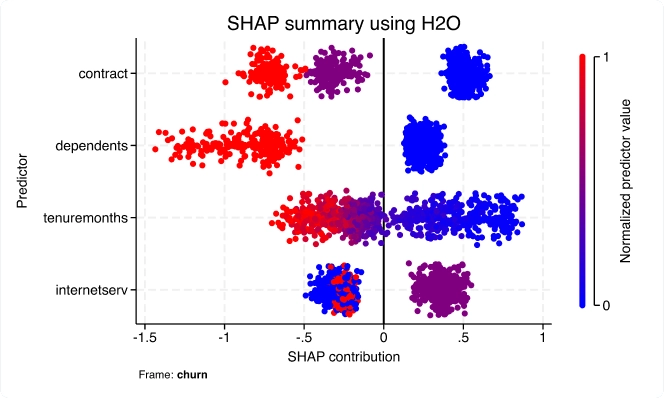
Machine learning via H2O: Ensemble decision trees
With the new h2oml suite, use machine learning via H2O to uncover insights from data when traditional statistical models fall short. Machine learning methods are often used to solve research and business problems focused on prediction.
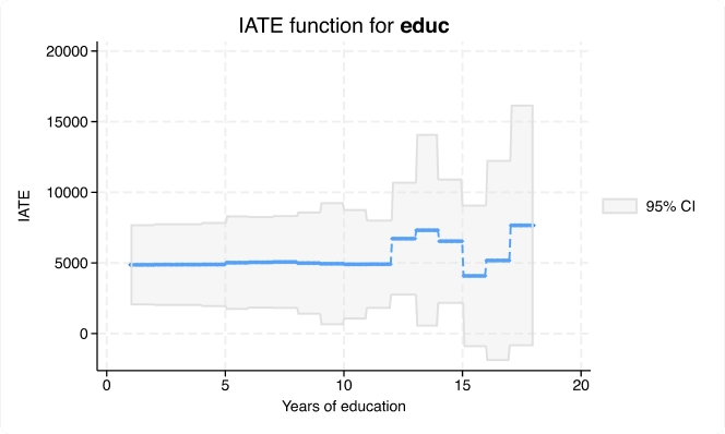
Conditional average treatment effects (CATE)
With the new cate command, you can go beyond estimating an overall treatment effect to estimating individualized or group-specific ones that address these types of research questions.
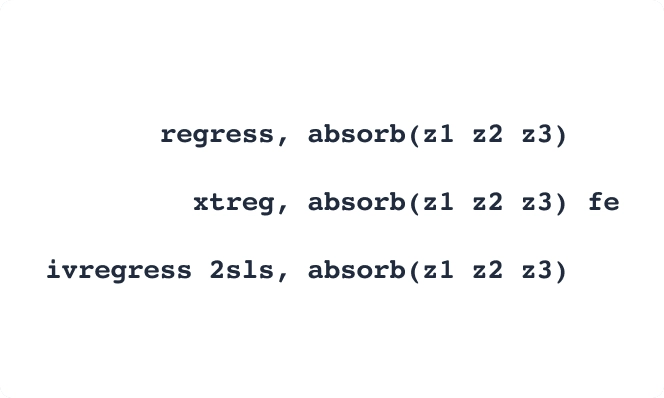
High-dimensional fixed effects (HDFE)
Absorb not just one but multiple high-dimensional categorical variables in your linear and fixed-effects linear models with option absorb() of commands areg and xtreg.
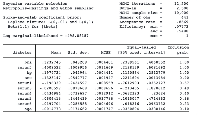
Bayesian variable selection for linear regression
With the new bayesselect command, you can perform Bayesian variable-selection for linear regression. This approach offers intuitive interpretation and stable inference, accounting for model uncertainty.
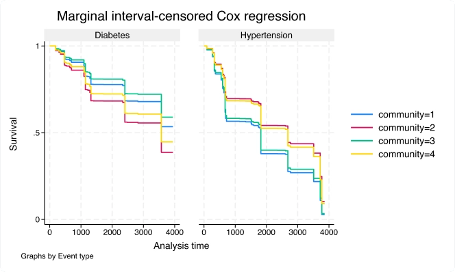
Marginal Cox PH models for interval-censored multiple- events data
Use the new stmgintcox command to analyse interval-censored multiple-event data.
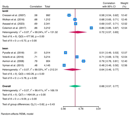
Meta-analysis for correlations
The meta suite now supports meta-analysis (MA) of a correlation coefficient. All standard meta-analysis features, such as forest plots and subgroup analysis, are supported.
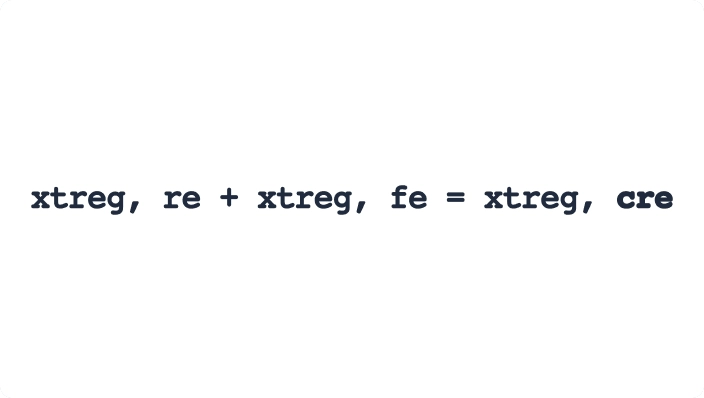
Correlated random-effects (CRE) model
Want coefficient estimates of time-invariant covariates in your panel-data model? With xtreg, cre, you can now fit a correlated random-effects model.
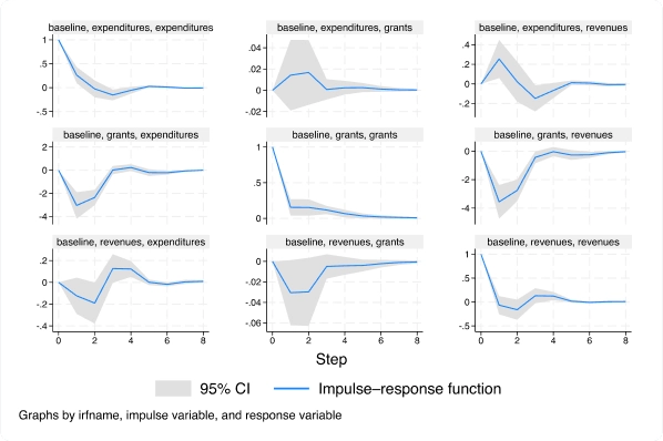
Panel-data vector autoregressive (VAR) model
With the new xtvar command, you can now fit a panel-data vector autoregressive (VAR) model to analyze the trajectories of related variables when you observe multiple units or panels over time.
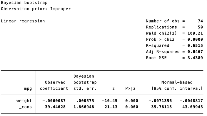
Bayesian bootstrap and replicate weights
You can use the new bayesboot prefix to perform Bayesian bootstrap of statistics produced by official and community-contributed commands. Bayesian bootstrap can incorporate prior information to obtain more precise parameter estimates.
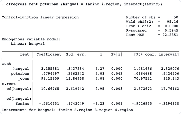
Control-function linear and probit models
Fit control-function linear and probit models with the new cfregress and cfprobit commands. Control-function models offer a more flexible approach to traditional instrumental-variables (IV) methods by including endogenous variables.
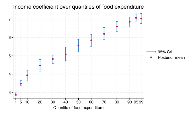
Bayesian quantile regression via asymmetric Laplace likelihood
The new bayes: qreg command fits Bayesian quantile regression. The Bayesian framework provides full posterior distributions for quantile regression coefficients that offer comprehensive inference.
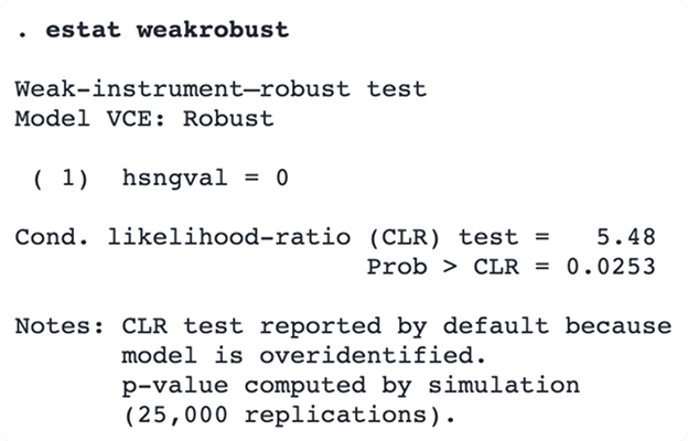
Inference robust to weak instruments
Use the new estat weakrobust command to perform reliable inference on endogenous regressors.
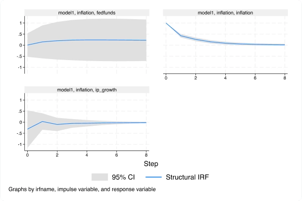
Structural vector autoregressive (SVAR) models via instrumental variables
With the new ivsvar command, you can use instruments instead of short-run constraints to estimate dynamic causal effects.
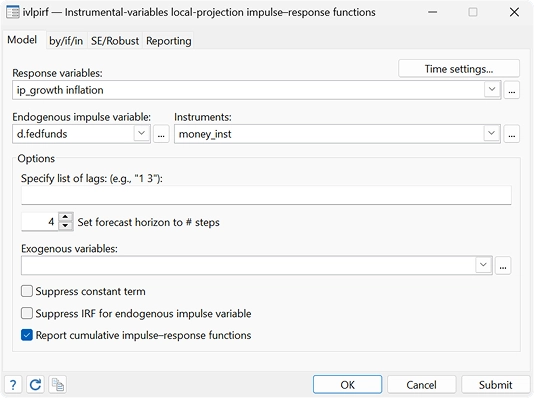
Instrumental-variables local-projection IRFs
With the new ivlpirf command, you can account for endogeneity when using local projections to estimate dynamic causal effects.

Mundlak specification test
Use the new estat mundlak postestimation command after xtreg to choose between random-effects (RE), fixed-effects (FE), or correlated random-effects (CRE) models even with cluster–robust, bootstrap, or jackknife standard errors.
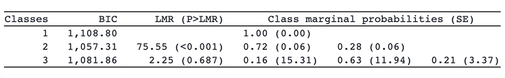
Latent class model-comparison statistics
With the new lcstats ncommand, you can use statistics such as entropy and a variety of information criteria, to help you determine the appropriate number of classes.
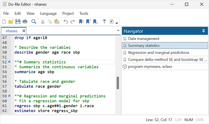
Do-file Editor: Autocompletion, templates, and more
The Do-file Editor has the following additions: Autocompletion of variable names, macros, and stored results; Code folding enhancements; Temporary and permanent bookmarks; Templates, tabs & Navigation panel.
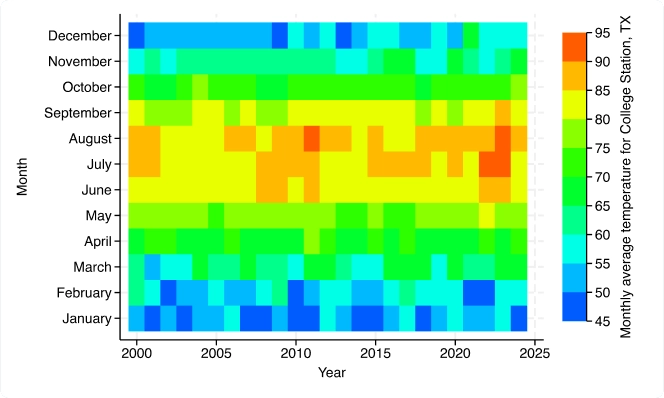
Graphics: Bar graph CIs, heat maps, and more
New graphics features: Heat maps (twoway); Range and point plot with capped spikes (twoway); Range and point plot with spikes (twoway); Improved labeling, CIs and Control of groupings for Bar Graphs, Dot Charts & Box Plots; Colors by variable for more graphs.
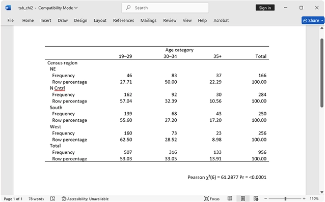
Tables: Easier tabulations, exporting, and more
Easily create and customize tables with titles, notes, and exporting for tables. The table command is a flexible tool for creating tabulations, tables of summary statistics, tables of regression results, and more.
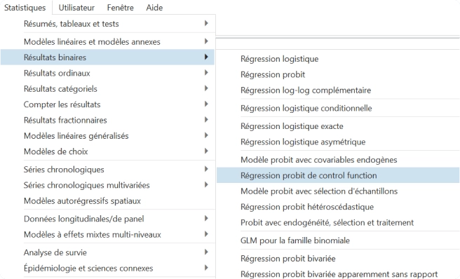
Stata in French
Stata's menus, dialogs, and the like can now be displayed in French. If your computer language is set to French (fr), Stata will automatically use its French setting.
Introducing StataNow™
New Features released at the speed of Stata. With StataNow, you will always have the latest features.
StataNow is a continuous-release version of Stata, offering new features as soon as they are ready and ensuring users always have access to the most recent version of Stata.
Straight from development to you. With StataNow, you always have access to the latest features.
What is StataNow?
First and foremost, StataNow is Stata. It is a continuous-release version of Stata that offers new features as soon as they are ready. StataNow is the result of our ongoing effort to deliver the best Stata-the most current Stata-to our users. Before StataNow, most new features became available only at the time of a major release such as Stata 17, Stata 18, and so on. StataNow provides access to new features sooner. For instance, StataNow contains features that will also be part of a future major release, Stata 20.
How can I get StataNow?
All annual license holders have access to StataNow, regardless of whether you have an annual license or multiyear license or whether your institution has a site license. You can access the latest StataNow features by simply typing update all in the Command window or asking your system administrator to update your Stata. Existing Stata 19 users may need to type update all twice. The first update will give you a Stata that knows how to update itself to StataNow. The second update will be StataNow. Then type help whatsnew to see the list of all features.
New users can obtain StataNow online, by purchasing any annual Stata license
If you have maintenance for your license, please contact us to obtain new download and license information for StataNow.
If you have a perpetual license without maintenance or your maintenance or license has expired, contact us for your options.
How do I know if I already have StataNow?
When you start Stata, you will see StataNow on the splash screen. You can also type about and you will see StataNow on the first line.
What's New in StataNow 19
Improved variable name truncation in the Data Editor
Released August 2025
In the Data Editor grid, you can now select whether variable names will be truncated at the end (the default), in the middle, or 1, 2, 3, or 4 characters before the end. You can change the truncation behavior in the Data Editor's preference dialog.
Local average treatment effects (LATE)
Released August 2025
StataNow™ introduces lateffects, a new feature for estimating local average treatment effects (LATE)—causal effects for the subpopulation that complies with treatment assignment.
When unobservable differences between treated and untreated units make identifying population-wide effects impossible, lateffects leverages an instrument—such as random assignment in experiments or an exogenous variable in observational studies—to isolate the effect for compliers.
Unlike standard two-stage least squares, which may fail when covariates are included, lateffects accurately estimates LATE both with and without covariates, providing a robust tool for causal inference in the presence of noncompliance.
VCE additions for linear models
Released August 2025
StataNow™ expands linear regression capabilities with more VCE options, giving you standard errors and confidence intervals that remain reliable in a wider range of scenarios.
New features include heteroskedasticity- and autocorrelation-consistent (HAC) standard errors for regress and areg, Driscoll–Kraay standard errors for xtreg, fe, and enhanced bias correction with HC2 and HC3 standard errors (including Hansen’s 2025 adjustment) across multiple commands.
ivregress now supports multiple nonnested clusters, and xtgls can model arbitrary within-panel correlation with corr(unstructured). These enhancements make robust inference easier and more flexible than ever.
Do-file Editor change history ribbon
Released August 2025
The Do-file Editor can now display the types of changes made to a document as colored markers in the change history ribbon, located in the margin. Two marker colors identify that the lines that have been modified and reverted to the original. To specify whether you want the change history ribbon to be visible, right-click in the Do-file Editor, select Preferences ..., and check/uncheck Change history in the General or Display tab.
Power analysis for logistic regression
Released May 2025
Designing an effective study requires balancing power, sample size, and cost. Stata's new power logistic command helps you determine the optimal sample size for logistic regression models without wasting time or resources.
Stata's power logistic command computes sample size, power, or effect size for the test of one coefficient of interest in a logistic regression model. As with all other powermethods, power logistic allows you to specify multiple values of parameters and automatically produce tabular and graphical results.
Stata in Your Research
Used by hundreds of thousands of researchers for more than 40 years, Stata provides everything you need for data science—data manipulation, visualization, statistics, and reproducible reporting.
Select your discipline and see how Stata can work for you.
Features For Data Scientists
Data wrangling
Scrape data from the web, import it from standard formats, or pull it in via SQL with JDBC or ODBC. Match-merge, link, append, reshape, transpose, sort, filter. Stata handles Unicode, frames (multiple datasets in memory), BLOBs, regular expressions, and more, whether working with hundreds of thousands or even billions of data points.
Automated reporting and customizable tables
Use Markdown to create Word documents and HTML files with embedded Stata code, output, and graphs. Automate Word, PDF, or Excel reports with both high-level export capabilities and low-level fine-grained programmatic access to automate production of the documents your team needs. Customize tables to clearly communicate results, and export your tables to Word, PDF, HTML, LaTeX, Excel, or Markdown.
Visualisation
Create graphs and customize them programmatically or interactively with the Graph Editor. Edits can even be recorded and "replayed" on other graphs for reproducibility. Export to industry standard formats suitable for web (SVG, PNG) or print (PDF, TIFF, EPS, PS).
Programming
Automate your entire workflow with both scripts and full-blown programming features like classes, structures, and pointers. A unique feature of Stata's programming environment is Mata, a fast and compiled matrix programming language. Of course, it has all the advanced matrix operations you need. It also has access to the power of LAPACK. What's more, it has built-in solvers and optimizers to make implementing your own estimator easier. And you can leverage all of Stata's estimation features and other features from within Mata.
PyStata—Python integration
Interact Stata code with Python code. You can seamlessly pass data and results between Stata and Python. You can use Stata within Jupyter Notebook and other IPython environments. You can call Python libraries such as NumPy, matplotlib, Scrapy, scikit-learn, and more from Stata. You can use Stata analyses from within Python.
Interoperability
Connect to external code via Python, Java, and C++ plugins. Write Python or Java code directly within your Stata code. Control Stata via Jupyter Notebook, OLE Automation, or call it in batch mode. Write custom SQL statements with JDBC and ODBC to extract from or populate databases. Access H2O clusters.
Statistics and modeling
Incorporate state-of-the-art statistical models and results in your workflow. Find groups in your data using unsupervised techniques including cluster analysis, principal components, factor analysis, multidimensional scaling, and correspondence analysis. Understand your groups even better using latent class analysis. When your analysis calls for supervised techniques, Stata has flexible nonparametric methods and an array of regression models from linear and logistic models to mixture models. Stata keeps up when your data call for special techniques. You have access to methods that understand and take advantage of the structure in time series, panel data, survival data, complex survey data, spatial data, and multilevel data. Stata provides the most approachable implementations of Bayesian methods and structural equation modeling available anywhere. You can request bootstrap methods for virtually any estimator. When your analysis calls for it, Stata automates other replication methods and simulations.
Reproducibility
Stata is the only software for data science and statistical analysis featuring a comprehensive version control system that ensures your code continues to run, unaltered, even after updates or new versions are released. No need to keep around multiple legacy installations to avoid breaking your system; Stata code from 25 years ago can still be run without modification. Datasets, graphs, scripts, programs, and more are 100% cross-platform and backward compatible.
Lasso
Use lasso and elastic net for model selection and prediction. And when you want to estimate effects and test coefficients for a few variables of interest, inferential methods provide estimates for these variables while using lassos to select from among a potentially large number of control variables. You can even account for endogenous covariates. Whether your goal is model selection, prediction, or inference, you can use Stata's lasso features with your continuous, binary, count, or time-to-event outcomes.
Features for Economists
Panel data
Take full advantage of the extra information that panel data provide while simultaneously handling the peculiarities of panel data. Study the time-invariant features within each panel, the relationships across panels, and how outcomes of interest change over time. Fit linear models or nonlinear models for binary, count, ordinal, censored, or survival outcomes with fixed-effects, random-effects, or population-averaged estimators. Fit dynamic models or models with endogeneity.
Time series
Handle the statistical challenges inherent to time-series data—autocorrelations, common factors, autoregressive conditional heteroskedasticity, unit roots, cointegration, and much more. Analyze univariate time series using ARIMA, ARFIMA, Markov-switching models, ARCH and GARCH models, and unobserved-components models. Compare ARIMA or ARFIMA models using AIC, BIC, and HQIC, and select the best number of autoregressive and moving-average terms. Analyze multivariate time series using VAR, structural VAR, VEC, multivariate GARCH, dynamic-factor models, and state-space models. Compute and graph impulse responses. Test for unit roots. Perform Bayesian time-series analysis.
Cross-sectional models
Fit classical linear models of the relationship between a continuous outcome, such as wage, and the determinants of wage, such as education level, age, experience, and economic sector. If your response is binary (for example, employed or unemployed), ordinal (education level), count (number of children), or censored (ticket sales in an existing venue), don't worry. Stata has maximum likelihood estimators—probit, ordered probit, Poisson, tobit, and many others—that estimate the relationship between such outcomes and their determinants. A vast array of tools is available to analyze such models. Predict outcomes and their confidence intervals. Test equality of parameters, or any linear or nonlinear combination of parameters.
Endogeneity and selection
When explanatory variables are related to omitted observable variables, or when they are related to unobservable variables, or when there is selection bias, then causal relationships are confounded and parameter estimates from standard estimators produce inconsistent estimates of the true relationships. Stata can fit consistent models when there is such endogeneity or selection—whether your outcome variable is continuous, binary, count, or ordinal and whether your data are cross-sectional or panel. Stata can even combine endogenous covariates, selection, and treatment effects in the same model.
Causal inference/Treatment effects
Estimate experimental-style causal effects from observational data; for instance, estimate the effect of a job training program on employment or the effect of a subsidy on production. Fit models for continuous, binary, count, fractional, and survival outcomes with binary or multivalued treatments using inverse-probability weighting (IPW), propensity-score matching, nearest-neighbor matching, regression adjustment, or doubly robust estimators. Fit models with exogenous or endogenous treatments. After estimation, test the overlap assumption and covariate balance. Add endogenous covariates and sample selection to some treatment-effects estimators. In the presence of group and time effects, you can use difference-in-differences (DID) and triple-differences (DDD) estimators. In the presence of high-dimensional covariates, you can use lasso. If causal effects are mediated through another variable, use causal mediation with mediate to disentangle direct and indirect effects.
Marginal effects and marginal means
Marginal effects and marginal means let you analyze and visualize the relationships between your outcome variable and your covariates, even when that outcome is binary, count, ordinal, categorical, or censored (tobit). Estimate population-averaged marginal effects or evaluate marginal effects at interesting or representative values of the covariates. Analyze the effect of interactions. You can even trace out the marginal effect over a range of interesting covariate values or covariate interactions. You can do all of this with marginal means (sometimes called potential-outcome means), even when your “mean” is a probability of a positive outcome or a count from a Poisson model. If you have panel data and random effects, these effects are automatically integrated out to provide marginal (that is, population-averaged) effects.
Choice models
Model your discrete choice data. If your outcome is, for instance, a choice to travel by bus, train, car, or airplane, you can fit a conditional logit, multinomial probit, or mixed logit model. Is your outcome instead a ranking of prefered travel methods? Fit a rank-ordered probit or rank-ordered logit model. Regardless of the model fit, you can use the margins to easily interpret the results. Estimate how much wait times at the airport affect the probability of traveling by air or even by train.
GMM
GMM (generalized method of moments) can be used to fit almost any statistical model, including both exactly identified and overidentified estimation problems. Overidentified problems arise when you have endogeneity, correlation in dynamic panels, sample selection, and many other situations. With Stata, you estimate these models by simply writing your moments and enclosing the parameters in curly braces. You can easily fit cross-sectional, time-series, panel-data, or survival-data models and test your overidentifying restrictions.
Demand systems
Fit demand systems to explore consumers' demand for goods and services. Given a budget and a bundle of goods and services, determine the expenditure and price elasticities for these goods. Choose between the Cobb–Douglas system, Stone's linear expenditure system, the translog indirect utility demand system, the almost ideal demand system (AIDS), the quadratic almost ideal demand system (QUAIDS), and others.
Lasso
Use lasso and elastic net for model selection and prediction. And when you want to estimate effects and test coefficients for a few variables of interest, inferential methods provide estimates for these variables while using lassos to select from among a potentially large number of control variables. You can even account for endogenous covariates. Whether your goal is model selection, prediction, or inference, you can use Stata's lasso features with your continuous, binary, count, or time-to-event outcomes.
Programming
Want to program your own commands to perform estimation, perform data management, or implement other new features? Stata is programmable, and thousands of Stata users have implemented and published thousands of community-contributed commands. These commands look and act just like official Stata commands and are easily installed for free over the Internet from within Stata. A unique feature of Stata's programming environment is Mata, a fast and compiled language with support for matrix types. Of course, it has all the advanced matrix operations you need. It also has access to the power of LAPACK. What's more, it has built-in solvers and optimizers to make implementing your own maximum likelihood, GMM, or other estimators easier. And you can leverage all of Stata's estimation and other features from within Mata. Many of Stata's official commands are themselves implemented in Mata.
PyStata - Python integration
Interact Stata code with Python code. You can seamlessly pass data and results between Stata and Python. You can use Stata within Jupyter Notebook and other IPython environments. You can call Python libraries such as NumPy, matplotlib, Scrapy, scikit-learn, and more from Stata. You can use Stata analyses from within Python.
Forecasting
Build multiequation models, and produce forecasts of levels, trends, rates, etc. Whether you have a small model with a few equations or a complete model of the economy with thousands of equations, Stata can help you build that model and produce forecasts. Your model can include both estimated relationships and known identities. You can easily create and compare forecasts under different scenarios, create static and dynamic forecasts, and even estimate stochastic confidence intervals. You can create your model by using an intuitive command syntax or by using the interactive forecasting control panel.
Survival Analysis
Analyze duration outcomes—outcomes measuring the time to an event such as failure or death—using Stata's specialized tools for survival analysis. Account for the complications inherent in survival data, such as sometimes not observing the event (right-, left-, and interval-censoring), individuals entering the study at differing times (delayed entry), and individuals who are not continuously observed throughout the study (gaps). You can estimate and plot the probability of survival over time. Or model survival as a function of covariates using Cox, Weibull, lognormal, and other regression models. Predict hazard ratios, mean survival time, and survival probabilities. Do you have groups of individuals in your study? Adjust for within-group correlation with a random-effects or shared-frailty model. If you have many potential covariates, use lasso cox and elasticnet cox for model selection and prediction.
Bayesian analysis
Perform Bayesian econometrics analysis using one of the Markov chain Monte Carlo (MCMC) methods. You can choose from various supported models, such as panel-data, hierarchical, VAR, and DSGE models, or you can even program your own. Extensive tools are available to check convergence, including multiple chains. Compute posterior mean estimates and credible intervals for model parameters and functions of model parameters. You can perform both interval- and model-based hypothesis testing. Compare models using Bayes factors. Compute model fit using posterior predictive values. Generate predictions and forecasts. If you want to account for model uncertainty in your regression model, use Bayesian model averaging.
Survey methods
Whether your data require a simple weighted adjustment because of differential sampling rates or you have data from a complex multistage survey, Stata's survey features can provide you with correct standard errors and confidence intervals for your inferences. Simply specify the relevant characteristics of your sampling design, such as sampling weights (including weights at multiple stages), clustering (at one, two, or more stages), stratification, and poststratification. After that, most of Stata's estimation commands can adjust their estimates to correct for your sampling design.
Meta-analysis
Combine results of multiple studies to estimate an overall effect. Use forest plots to visualize results. Use subgroup analysis and meta-regression to explore study heterogeneity. Use funnel plots and formal tests to explore publication bias and small-study effects. Use trim-and-fill analysis to assess the impact of publication bias on results. Perform cumulative and leave-one-out meta-analysis. Perform univariate, multilevel, and multivariate meta-analysis. Use the meta suite, or let the Control Panel interface guide you through your entire meta-analysis.
Automated reporting and customizable tables
Stata is designed for reproducible research, including the ability to create dynamic documents incorporating your analysis results. Create Word or PDF files, populate Excel worksheets with results and format them to your liking, and mix Markdown, HTML, Stata results, and Stata graphs, all from within Stata. Create tables that compare regression results or summary statistics, use default styles or apply your own, and export your tables to Word, PDF, HTML, LaTeX, Excel, or Markdown and include them in your reports.
Features for Education
Multilevel mixed-effects models
Whether the groupings in your data arise in a nested fashion (students nested in classrooms and classrooms nested in schools) or in a nonnested fashion (elementary school crossed with middle school), you can fit a multilevel model to account for the lack of independence within these groups. Fit models for continuous, binary, count, ordinal, and survival outcomes. Estimate variances of random intercepts and random coefficients. Compute intraclass correlations. Predict random effects. Estimate relationships that are population averaged over the random effects.
Structural equation modeling (SEM)
Estimate mediation effects, analyze the relationship between an unobserved latent concept such as verbal abilities and the observed variables that measure verbal abilities, or fit a model with complex relationships among both latent and observed variables. Fit models with continuous, binary, count, and ordinal outcomes. Even fit hierarchical models with groups of correlated observations such as children within the same schools. Evaluate model fit. Compute indirect and total effects. Fit models by drawing a path diagram or using the straightforward command syntax.
General Linear Models
Fit one- and two-way models. Or fit models with three, four, or even more factors. Analyze data with nested factors, with fixed and random factors, or with repeated measures. Use ANCOVA models when you have continuous covariates and MANOVA models when you have multiple outcome variables. Further explore the relationships between your outcome and predictors by estimating effect sizes and computing least-squares and marginal means. Perform contrasts and pairwise comparisons. Analyze and plot interactions.
IRT (item response theory)
Explore the relationship between unobserved latent characteristics such as mathematical aptitude and the probability of correctly answering test questions (items). Or explore the relationship between teacher job satisfaction and self-reported responses to questions related to job statisfaction. IRT can be used to create measures of such unobserved traits or place individuals on a scale measuring the trait. It can also be used to select the best items for measuring a latent trait. IRT models are available for binary, graded, rated, partial-credit, and nominal response items. Visualize the relationships using item characteristic curves, and measure overall test performance using test information functions.
Linear, binary and count regressions
Fit classical linear regression models of the relationship between a continuous outcome, such as a reading test score, and the determinants of the score, such as teaching method and the student's reading level in the previous grade. If your response is binary (for example, pass or fail test), ordinal (education level), count (number of students), or categorical (private, public, or home school), don't worry. Stata has maximum likelihood estimators—logistic, ordered logistic, Poisson, multinomial logit, and many others—that estimate the relationship between such outcomes and their determinants. A vast array of tools is available after fitting such models. Predict outcomes and their confidence intervals. Test equality of parameters. Compute linear and nonlinear combinations of parameters.
Linear, binary and count regressions
Account for missing data in your sample using multiple imputation. Choose from univariate and multivariate methods to impute missing values in continuous, censored, truncated, binary, ordinal, categorical, and count variables. Then, in a single step, estimate parameters using the imputed datasets, and combine results. Fit a linear model, logit model, Poisson model, hierarchical model, survival model, or one of the many other supported models. Use the mi command, or let the Control Panel interface guide you through your entire MI analysis.
Choice models
Model your discrete choice data. If your outcome is, for instance, a choice to travel by bus, train, car, or airplane, you can fit a conditional logit, multinomial probit, or mixed logit model. Is your outcome instead a ranking of prefered travel methods? Fit a rank-ordered probit or rank-ordered logit model. Regardless of the model fit, you can use the margins to easily interpret the results. Estimate how much wait times at the airport affect the probability of traveling by air or even by train.
Contrasts, marginal means and profile plots
Quickly and easily obtain contrasts for categorical variables and their interactions. R.edlevel will give you all the contrasts of education level with a reference category. A.edlevel will give you each paired contrast with the next higher education level. There are many more named contrasts, and you can specify your own. If you don't like typing, use a dialog box to select your contrasts. Marginal means are just a simple command or mouse click away after almost any estimation command. Evaluating interaction effects, the effects of moderating variables, is just as easy. And this is not just for linear models, but for models with binary, ordinal, and count outcomes. Even for hierarchical models with correct handling of random effects. A simple command or a few mouse clicks will get you a profile plot of any of these results.
Power, precision and sample size
Before you conduct your experiment, determine the sample size needed to detect meaningful effects without wasting resources. Do you intend to compute CIs for means or variances or perform tests for proportions or correlations? Do you plan to fit a Cox proportional hazards model or compare survivor functions using a log-rank test? Do you want to use a Cochran—Mantel—Haenszel test of association or a Cochran—Armitage trend test? Use Stata's power command to compute power and sample size, create customized tables, and automatically graph the relationships between power, sample size, and effect size for your planned study. Or use the ciwidth command to do the same but for CIs instead of hypothesis tests by computing the required sample size for the desired CI precision. Or use gsdesign to compute stopping boundaries and the required sample sizes for group sequential designs. Instead of commands, use the interactive Control Panel to perform your analysis.
Causal Inference
Estimate experimental-style causal effects from observational data. With Stata's treatment-effects estimators, you can use a potential-outcomes (counterfactuals) framework to estimate, for instance, the effect of family structure on child development or the effect of unemployment on anxiety. Fit models for continuous, binary, count, fractional, and survival outcomes with binary or multivalued treatments using inverse-probability weighting (IPW), propensity-score matching, nearest-neighbor matching, regression adjustment, or doubly robust estimators. If the assignment to a treatment is not independent of the outcome, you can use an endogenous treatment-effects estimator. In the presence of group and time effects, you can use difference-in-differences (DID) and triple-differences (DDD) estimators. In the presence of high-dimensional covariates, you can use lasso. If causal effects are mediated through another variable, use causal mediation with mediate to disentangle direct and indirect effects.
Multivariate methods
Use multivariate analyses to evaluate relationships among variables from many different perspectives. Perform multivariate tests of means, or fit multivariate regression and MANOVA models. Explore relationships between two sets of variables, such as aptitude measurements and achievement measurements, using canonical correlation. Examine the number and structure of latent concepts underlying a set of variables using exploratory factor analysis. Or use principal component analysis to find underlying structure or to reduce the number of variables used in a subsequent analysis. Discover groupings of observations in your data using cluster analysis. If you have known groups in your data, describe differences between them using discriminant analysis.
Automated reporting and customizable tables
Stata is designed for reproducible research, including the ability to create dynamic documents incorporating your analysis results. Create Word or PDF files, populate Excel worksheets with results and format them to your liking, and mix Markdown, HTML, Stata results, and Stata graphs, all from within Stata. Create tables that compare regression results or summary statistics, use default styles or apply your own, and export your tables to Word, PDF, HTML, LaTeX, Excel, or Markdown and include them in your reports.
Bayesian analysis
Perform Bayesian econometrics analysis using one of the Markov chain Monte Carlo (MCMC) methods. You can choose from various supported models, such as panel-data, hierarchical, VAR, and DSGE models, or you can even program your own. Extensive tools are available to check convergence, including multiple chains. Compute posterior mean estimates and credible intervals for model parameters and functions of model parameters. You can perform both interval- and model-based hypothesis testing. Compare models using Bayes factors. Compute model fit using posterior predictive values. Generate predictions and forecasts. If you want to account for model uncertainty in your regression model, use Bayesian model averaging.
Meta-analysis
Combine results of multiple studies to estimate an overall effect. Use forest plots to visualize results. Use subgroup analysis and meta-regression to explore study heterogeneity. Use funnel plots and formal tests to explore publication bias and small-study effects. Use trim-and-fill analysis to assess the impact of publication bias on results. Perform cumulative and leave-one-out meta-analysis. Perform univariate, multilevel, and multivariate meta-analysis. Use the meta suite, or let the Control Panel interface guide you through your entire meta-analysis.
Jupyter Notebook with Stata
Jupyter Notebook is widely used by researchers and scientists to share their ideas and results for collaboration and innovation. It is an easy-to-use web application that allows you to combine code, visualizations, mathematical formulas, narrative text, and other rich media in a single document (a "notebook") for interactive computing and developing. You can invoke Stata and Mata from Jupyter Notebook with the IPython (interactive Python) kernel. This means you can combine the capabilities of both Python and Stata in a single environment to make your work easily reproducible and shareable with others.
Features for Epidemiologists
Epidemiological tables
Want to analyze data from a prospectiv321 laddence") study, cohort study, case–control study, or matched case–control study? Stata's tables for epidemiologists make it easy to summarize your data and compute statistics such as incidence-rate ratios, incidence-rate differences, risk ratios, risk differences, odds ratios, and attributable fractions. You can analyze stratified data too—compute Mantel–Haenszel combined estimates, perform tests of homogeneity, and standardize estimates. If you have an ordinal rather than binary exposure, you can perform a test for a trend.
Survival analysis
Analyze duration outcomes—outcomes measuring the time to an event such as failure or death—using Stata's specialized tools for survival analysis. Account for the complications inherent in survival data, such as sometimes not observing the event (right-, left-, and interval-censoring), individuals entering the study at differing times (delayed entry), and individuals who are not continuously observed throughout the study (gaps). You can estimate and plot the probability of survival over time. Or model survival as a function of covariates using Cox, Weibull, lognormal, and other regression models. Predict hazard ratios, mean survival time, and survival probabilities. Do you have groups of individuals in your study? Adjust for within-group correlation with a random-effects or shared-frailty model. If you have many potential covariates, use lasso cox and elasticnet cox for model selection and prediction.
Linear, binary and count regressions
Fit classical ANOVA and linear regression models of the relationship between a continuous outcome, such as weight, and the determinants of weight, such as height, diet, and level of exercise. If your response is binary, ordinal, categorical, or count, don't worry. Stata has estimators for these types of outcomes too. Use logistic regression to adjust odds ratios for confounding variables. Estimate incidence rates using a Poisson model. Analyze matched case–control data with conditional logistic regression. A vast array of tools is available after fitting such models. Predict outcomes and their confidence intervals. Test equality of parameters. Compute linear and nonlinear combinations of parameters.
Survey methods
Whether your data require a simple weighted adjustment because of differential sampling rates or you have data from a complex multistage survey, Stata's survey features can provide you with correct standard errors and confidence intervals for your inferences. Simply specify the relevant characteristics of your sampling design, such as sampling weights (including weights at multiple stages), clustering (at one, two, or more stages), stratification, and poststratification. After that, most of Stata's estimation commands can adjust their estimates to correct for your sampling design.
Marginal means, contrasts and interactions
Marginal means and contrasts let you analyze the relationships between your outcome variable and your predictors, even when your outcome is binary, count, ordinal, or categorical. For instance, after you fit a logistic regression of a disease on an exposure variable and other covariates, your marginal means may be population-averaged risks. Or you can set the covariates to interesting values to compute adjusted risks and then use contrasts to get adjusted risk differences. After fitting almost any model in Stata, you can analyze the effect of covariate interactions and easily create plots to visualize those interactions.
Power, precision and sample size
Before you conduct your experiment, determine the sample size needed to detect meaningful effects without wasting resources. Do you intend to compute CIs for means or variances or perform tests for proportions or correlations? Do you plan to fit a Cox proportional hazards model or compare survivor functions using a log-rank test? Do you want to use a Cochran—Mantel—Haenszel test of association or a Cochran—Armitage trend test? Use Stata's power command to compute power and sample size, create customized tables, and automatically graph the relationships between power, sample size, and effect size for your planned study. Or use the ciwidth command to do the same but for CIs instead of hypothesis tests by computing the required sample size for the desired CI precision. Or use gsdesign to compute stopping boundaries and the required sample sizes for group sequential designs. Instead of commands, use the interactive Control Panel to perform your analysis.
Meta-analysis
Combine results of multiple studies to estimate an overall effect. Use forest plots to visualize results. Use subgroup analysis and meta-regression to explore study heterogeneity. Use funnel plots and formal tests to explore publication bias and small-study effects. Use trim-and-fill analysis to assess the impact of publication bias on results. Perform cumulative and leave-one-out meta-analysis. Perform univariate, multilevel, and multivariate meta-analysis. Use the meta suite, or let the Control Panel interface guide you through your entire meta-analysis.
Causal inference
Estimate experimental-style causal effects from observational data. With Stata's treatment-effects estimators, you can use a potential-outcomes (counterfactuals) framework to estimate, for instance, the effect of family structure on child development or the effect of unemployment on anxiety. Fit models for continuous, binary, count, fractional, and survival outcomes with binary or multivalued treatments using inverse-probability weighting (IPW), propensity-score matching, nearest-neighbor matching, regression adjustment, or doubly robust estimators. If the assignment to a treatment is not independent of the outcome, you can use an endogenous treatment-effects estimator. In the presence of group and time effects, you can use difference-in-differences (DID) and triple-differences (DDD) estimators. In the presence of high-dimensional covariates, you can use lasso. If causal effects are mediated through another variable, use causal mediation with mediate to disentangle direct and indirect effects.
Multiple imputation
Account for missing data in your sample using multiple imputation. Choose from univariate and multivariate methods to impute missing values in continuous, censored, truncated, binary, ordinal, categorical, and count variables. Then, in a single step, estimate parameters using the imputed datasets, and combine results. Fit a linear model, logit model, Poisson model, multilevel model, survival model, or one of the many other supported models. Use the mi command, or let the Control Panel interface guide you through your entire MI analysis.
Multilevel mixed-effects models
Whether the groupings in your data arise in a nested fashion (patients nested in clinics and clinics nested in regions) or in a nonnested fashion (regions crossed with occupations), you can fit a multilevel model to account for the lack of independence within these groups. Fit models for continuous, binary, count, ordinal, and survival outcomes. Estimate variances of random intercepts and random coefficients. Compute intraclass correlations. Predict random effects. Estimate relationships that are population averaged over the random effects.
Bayesian analysis
Fit Bayesian regression models using one of the Markov chain Monte Carlo (MCMC) methods. You can choose from various supported models or even program your own. Extensive tools are available to check convergence, including multiple chains. Compute posterior mean estimates and credible intervals for model parameters and functions of model parameters. You can perform both interval- and model-based hypothesis testing. Compare models using Bayes factors. Compute model fit using posterior predictive values and generate predictions. If you want to account for model uncertainty in your regression model, use Bayesian model averaging.
Additive models of relative risk
Determine how exposures interact to put subjects at a higher risk of experiencing an outcome of interest. For example, you might be investigating how exposure to cigarette smoke and asbestos interact to increase the risk of lung cancer. With Stata's reri command, you can measure two–way interactions in an additive model of relative risk, while accounting for other risk factors. Choose from various supported models, such as binomial generalized linear, Poisson, negative binomial, logistic, Cox, parametric survival, and interval–censored parametric and semiparametric survival models. Estimate the relative excess risk due to interaction (RERI), attributable proportion (AP), and synergy index (SI).
Automated reporting and customizable tables
Stata is designed for reproducible research, including the ability to create dynamic documents incorporating your analysis results. Create Word or PDF files, populate Excel worksheets with results and format them to your liking, and mix Markdown, HTML, Stata results, and Stata graphs, all from within Stata. Create tables that compare regression results or summary statistics, use default styles or apply your own, and export your tables to Word, PDF, HTML, LaTeX, Excel, or Markdown and include them in your reports.
Jupyter Notebook with Stata
Jupyter Notebook is widely used by researchers and scientists to share their ideas and results for collaboration and innovation. It is an easy-to-use web application that allows you to combine code, visualizations, mathematical formulas, narrative text, and other rich media in a single document (a "notebook") for interactive computing and developing. You can invoke Stata and Mata from Jupyter Notebook with the IPython (interactive Python) kernel. This means you can combine the capabilities of both Python and Stata in a single environment to make your work easily reproducible and shareable with others.
Features for Biostatisticians
Survival analysis
Analyze duration outcomes—outcomes measuring the time to an event such as failure or death—using Stata's specialized tools for survival analysis. Account for the complications inherent in survival data, such as sometimes not observing the event (right-, left-, and interval-censoring), individuals entering the study at differing times (delayed entry), and individuals who are not continuously observed throughout the study (gaps). You can estimate and plot the probability of survival over time. Or model survival as a function of covariates using Cox, Weibull, lognormal, and other regression models. Predict hazard ratios, mean survival time, and survival probabilities. Do you have groups of individuals in your study? Adjust for within-group correlation with a random-effects or shared-frailty model. If you have many potential covariates, use lasso cox and elasticnet cox for model selection and prediction.
Multilevel mixed-effects models
Whether the groupings in your data arise in a nested fashion (patients nested in clinics and clinics nested in regions) or in a nonnested fashion (regions crossed with occupations), you can fit a multilevel model to account for the lack of independence within these groups. Fit models for continuous, binary, count, ordinal, and survival outcomes. Estimate variances of random intercepts and random coefficients. Compute intraclass correlations. Predict random effects. Estimate relationships that are population averaged over the random effects.
Bayesian analysis
Fit Bayesian regression models using one of the Markov chain Monte Carlo (MCMC) methods. You can choose from various supported models or even program your own. Extensive tools are available to check convergence, including multiple chains. Compute posterior mean estimates and credible intervals for model parameters and functions of model parameters. You can perform both interval- and model-based hypothesis testing. Compare models using Bayes factors. Compute model fit using posterior predictive values and generate predictions. If you want to account for model uncertainty in your regression model, use Bayesian model averaging.
Power, precision and sample size
Before you conduct your experiment, determine the sample size needed to detect meaningful effects without wasting resources. Do you intend to compute CIs for means or variances or perform tests for proportions or correlations? Do you plan to fit a Cox proportional hazards model or compare survivor functions using a log-rank test? Do you want to use a Cochran—Mantel—Haenszel test of association or a Cochran—Armitage trend test? Use Stata's power command to compute power and sample size, create customized tables, and automatically graph the relationships between power, sample size, and effect size for your planned study. Or use the ciwidth command to do the same but for CIs instead of hypothesis tests by computing the required sample size for the desired CI precision. Or use gsdesign to compute stopping boundaries and the required sample sizes for group sequential designs. Instead of commands, use the interactive Control Panel to perform your analysis.
Linear, binary and count regressions
Fit classical ANOVA and linear regression models of the relationship between a continuous outcome, such as weight, and the determinants of weight, such as height, diet, and level of exercise. If your response is binary, ordinal, categorical, or count, don't worry. Stata has estimators for these types of outcomes too. Use logistic regression to estimate odds ratios. Estimate incidence rates using a Poisson model. Analyze matched case–control data with conditional logistic regression. A vast array of tools is available after fitting such models. Predict outcomes and their confidence intervals. Test equality of parameters. Compute linear and nonlinear combinations of parameters.
Meta-analysis
Combine results of multiple studies to estimate an overall effect. Use forest plots to visualize results. Use subgroup analysis and meta-regression to explore study heterogeneity. Use funnel plots and formal tests to explore publication bias and small-study effects. Use trim-and-fill analysis to assess the impact of publication bias on results. Perform cumulative and leave-one-out meta-analysis. Perform univariate, multilevel, and multivariate meta-analysis. Use the meta suite, or let the Control Panel interface guide you through your entire meta-analysis.
Multiple imputation
Account for missing data in your sample using multiple imputation. Choose from univariate and multivariate methods to impute missing values in continuous, censored, truncated, binary, ordinal, categorical, and count variables. Then, in a single step, estimate parameters using the imputed datasets, and combine results. Fit a linear model, logit model, Poisson model, hierarchical model, survival model, or one of the many other supported models. Use the mi command, or let the Control Panel interface guide you through your entire MI analysis.
Marginal means, contrasts and interactions
Marginal means and contrasts let you analyze the relationships between your outcome variable and your covariates, even when that outcome is binary, count, ordinal, categorical, or survival. Compute adjusted predictions with covariates set to interesting or representative values. Or compute marginal means for each level of a categorical covariate. Make comparisons of the adjusted predictions or marginal means using contrasts. If you have multilevel data and random effects, these effects are automatically integrated out to provide marginal (that is, population-averaged) estimates. After fitting almost any model in Stata, analyze the effect of covariate interactions, and easily create plots to visualize those interactions.
Causal inference
Estimate experimental-style causal effects from observational data. With Stata's treatment-effects estimators, you can use a potential-outcomes (counterfactuals) framework to estimate, for instance, the effect of family structure on child development or the effect of unemployment on anxiety. Fit models for continuous, binary, count, fractional, and survival outcomes with binary or multivalued treatments using inverse-probability weighting (IPW), propensity-score matching, nearest-neighbor matching, regression adjustment, or doubly robust estimators. If the assignment to a treatment is not independent of the outcome, you can use an endogenous treatment-effects estimator. In the presence of group and time effects, you can use difference-in-differences (DID) and triple-differences (DDD) estimators. In the presence of high-dimensional covariates, you can use lasso. If causal effects are mediated through another variable, use causal mediation with mediate to disentangle direct and indirect effects.
Epidemiological tables
Want to analyze data from a prospective (incidence) study, cohort study, case–control study, or matched case–control study? Stata's tables for epidemiologists make it easy to summarize your data and compute statistics such as incidence-rate ratios, incidence-rate differences, risk ratios, risk differences, odds ratios, and attributable fractions. You can analyze stratified data too—compute Mantel–Haenszel combined estimates, perform tests of homogeneity, and standardize estimates. If you have an ordinal rather than binary exposure, you can perform a test for a trend.
Programming
Want to program your own commands to perform estimation, perform data management, or implement other new features? Stata is programmable, and thousands of Stata users have implemented and published thousands of community-contributed commands. These commands look and act just like official Stata commands and are easily installed for free over the Internet from within Stata. A unique feature of Stata's programming environment is Mata, a fast and compiled language with support for matrix types. Of course, it has all the advanced matrix operations you need. It also has access to the power of LAPACK. What's more, it has built-in solvers and optimizers to make implementing your own maximum likelihood, GMM, or other estimators easier. And you can leverage all of Stata's estimation and other features from within Mata. Many of Stata's official commands are themselves implemented in Mata.
PyStata - Python integration
Interact Stata code with Python code. You can seamlessly pass data and results between Stata and Python. You can use Stata within Jupyter Notebook and other IPython environments. You can call Python libraries such as NumPy, matplotlib, Scrapy, scikit-learn, and more from Stata. You can use Stata analyses from within Python.
Automated reporting and customizable tables
Stata is designed for reproducible research, including the ability to create dynamic documents incorporating your analysis results. Create Word or PDF files, populate Excel worksheets with results and format them to your liking, and mix Markdown, HTML, Stata results, and Stata graphs, all from within Stata. Create tables that compare regression results or summary statistics, use default styles or apply your own, and export your tables to Word, PDF, HTML, LaTeX, Excel, or Markdown and include them in your reports.
Features for Medical Researchers
General linear models
Fit one- and two-way models. Or fit models with three, four, or even more factors. Analyze data with nested factors, with fixed and random factors, or with repeated measures. Use ANCOVA models when you have continuous covariates and MANOVA models when you have multiple outcome variables. Further explore the relationships between your outcome and predictors by estimating effect sizes and computing least-squares and marginal means. Perform contrasts and pairwise comparisons. Analyze and plot interactions.
Linear, binary and count regressions
Fit classical ANOVA and linear regression models of the relationship between a continuous outcome, such as weight, and the determinants of weight, such as height, diet, and level of exercise. If your response is binary, ordinal, categorical, or count, don't worry. Stata has estimators for these types of outcomes too. Use logistic regression to estimate odds ratios. Estimate incidence rates using a Poisson model. Analyze matched case–control data with conditional logistic regression. A vast array of tools is available after fitting such models. Predict outcomes and their confidence intervals. Test equality of parameters. Compute linear and nonlinear combinations of parameters.
Power, precision and sample size
Before you conduct your experiment, determine the sample size needed to detect meaningful effects without wasting resources. Do you intend to compute CIs for means or variances or perform tests for proportions or correlations? Do you plan to fit a Cox proportional hazards model or compare survivor functions using a log-rank test? Do you want to use a Cochran—Mantel—Haenszel test of association or a Cochran—Armitage trend test? Use Stata's power command to compute power and sample size, create customized tables, and automatically graph the relationships between power, sample size, and effect size for your planned study. Or use the ciwidth command to do the same but for CIs instead of hypothesis tests by computing the required sample size for the desired CI precision. Or use gsdesign to compute stopping boundaries and the required sample sizes for group sequential designs. Instead of commands, use the interactive Control Panel to perform your analysis.
Marginal means, contrasts and interactions
Marginal means and contrasts let you analyze the relationships between your outcome variable and your covariates, even when that outcome is binary, count, ordinal, categorical, or survival. Compute adjusted predictions with covariates set to interesting or representative values. Or compute marginal means for each level of a categorical covariate. Make comparisons of the adjusted predictions or marginal means using contrasts. If you have multilevel data and random effects, these effects are automatically integrated out to provide marginal (that is, population-averaged) estimates. After fitting almost any model in Stata, analyze the effect of covariate interactions, and easily create plots to visualize those interactions.
Multilevel mixed-effects models
Whether the groupings in your data arise in a nested fashion (patients nested in clinics and clinics nested in regions) or in a nonnested fashion (regions crossed with occupations), you can fit a multilevel model to account for the lack of independence within these groups. Fit models for continuous, binary, count, ordinal, and survival outcomes. Estimate variances of random intercepts and random coefficients. Compute intraclass correlations. Predict random effects. Estimate relationships that are population averaged over the random effects.
Meta-analysis
Combine results of multiple studies to estimate an overall effect. Use forest plots to visualize results. Use subgroup analysis and meta-regression to explore study heterogeneity. Use funnel plots and formal tests to explore publication bias and small-study effects. Use trim-and-fill analysis to assess the impact of publication bias on results. Perform cumulative and leave-one-out meta-analysis. Perform univariate, multilevel, and multivariate meta-analysis. Use the meta suite, or let the Control Panel interface guide you through your entire meta-analysis.
Multiple imputation
Account for missing data in your sample using multiple imputation. Choose from univariate and multivariate methods to impute missing values in continuous, censored, truncated, binary, ordinal, categorical, and count variables. Then, in a single step, estimate parameters using the imputed datasets, and combine results. Fit a linear model, logit model, Poisson model, hierarchical model, survival model, or one of the many other supported models. Use the mi command, or let the Control Panel interface guide you through your entire MI analysis.
Survival analysis
Analyze duration outcomes—outcomes measuring the time to an event such as failure or death—using Stata's specialized tools for survival analysis. Account for the complications inherent in survival data, such as sometimes not observing the event (right-, left-, and interval-censoring), individuals entering the study at differing times (delayed entry), and individuals who are not continuously observed throughout the study (gaps). You can estimate and plot the probability of survival over time. Or model survival as a function of covariates using Cox, Weibull, lognormal, and other regression models. Predict hazard ratios, mean survival time, and survival probabilities. Do you have groups of individuals in your study? Adjust for within-group correlation with a random-effects or shared-frailty model. If you have many potential covariates, use lasso cox and elasticnet cox for model selection and prediction.
Epidemiological tables
Want to analyze data from a prospective (incidence) study, cohort study, case–control study, or matched case–control study? Stata's tables for epidemiologists make it easy to summarize your data and compute statistics such as incidence-rate ratios, incidence-rate differences, risk ratios, risk differences, odds ratios, and attributable fractions. You can analyze stratified data too—compute Mantel–Haenszel combined estimates, perform tests of homogeneity, and standardize estimates. If you have an ordinal rather than binary exposure, you can perform a test for a trend.
Additive models of relative risk
Determine how exposures interact to put subjects at a higher risk of experiencing an outcome of interest. For example, you might be investigating how exposure to cigarette smoke and asbestos interact to increase the risk of lung cancer. With Stata's reri command, you can measure two–way interactions in an additive model of relative risk, while accounting for other risk factors. Choose from various supported models, such as binomial generalized linear, Poisson, negative binomial, logistic, Cox, parametric survival, and interval–censored parametric and semiparametric survival models. Estimate the relative excess risk due to interaction (RERI), attributable proportion (AP), and synergy index (SI).
Automated reporting and customizable tables
Stata is designed for reproducible research, including the ability to create dynamic documents incorporating your analysis results. Create Word or PDF files, populate Excel worksheets with results and format them to your liking, and mix Markdown, HTML, Stata results, and Stata graphs, all from within Stata. Create tables that compare regression results or summary statistics, use default styles or apply your own, and export your tables to Word, PDF, HTML, LaTeX, Excel, or Markdown and include them in your reports.
Jupyter Notebook with Stata
Jupyter Notebook is widely used by researchers and scientists to share their ideas and results for collaboration and innovation. It is an easy-to-use web application that allows you to combine code, visualizations, mathematical formulas, narrative text, and other rich media in a single document (a "notebook") for interactive computing and developing. You can invoke Stata and Mata from Jupyter Notebook with the IPython (interactive Python) kernel. This means you can combine the capabilities of both Python and Stata in a single environment to make your work easily reproducible and shareable with others.
Features for Sociologists
Survey methods
Whether your data require a simple weighted adjustment because of differential sampling rates or you have data from a complex multistage survey, Stata's survey features can provide you with correct standard errors and confidence intervals for your inferences. Simply specify the relevant characteristics of your sampling design, such as sampling weights (including weights at multiple stages), clustering (at one, two, or more stages), stratification, and poststratification. After that, most of Stata's estimation commands can adjust their estimates to correct for your sampling design.
Multiple imputation
Account for missing data in your sample using multiple imputation. Choose from univariate and multivariate methods to impute missing values in continuous, censored, truncated, binary, ordinal, categorical, and count variables. Then, in a single step, estimate parameters using the imputed datasets, and combine results. Fit a linear model, logit model, Poisson model, multilevel model, survival model, or one of the many other supported models. Use the mi command, or let the Control Panel interface guide you through your entire MI analysis.
Multilevel mixed-effects models
Whether the groupings in your data arise in a nested fashion (students nested in schools and schools nested in districts) or in a nonnested fashion (regions crossed with occupations), you can fit a multilevel model to account for the lack of independence within these groups. Fit models for continuous, binary, count, ordinal, and survival outcomes. Estimate variances of random intercepts and random coefficients. Compute intraclass correlations. Predict random effects. Estimate relationships that are population averaged over the random effects.
Panel data
Take full advantage of the extra information that panel data provide while simultaneously handling the peculiar difficulties that panel data present. Study the time-invariant idiosyncratic features within each panel, the relationships across panels, and how outcomes of interest change over time. Fit linear models or nonlinear models for binary, count, ordinal, censored, or survival outcomes with fixed-effects, random-effects, or population-averaged estimators. Fit dynamic models or models with endogeneity. Fit Bayesian panel-data models.
Meta-analysis
Combine results of multiple studies to estimate an overall effect. Use forest plots to visualize results. Use subgroup analysis and meta-regression to explore study heterogeneity. Use funnel plots and formal tests to explore publication bias and small-study effects. Use trim-and-fill analysis to assess the impact of publication bias on results. Perform cumulative and leave-one-out meta-analysis. Perform univariate, multilevel, and multivariate meta-analysis. Use the meta suite, or let the Control Panel interface guide you through your entire meta-analysis.
Linear, binary and count regressions
Fit classical linear models of the relationship between a continuous outcome, such as wage, and the determinants of wage, such as education level, age, experience, and economic sector. If your response is binary (for example, employed or unemployed), ordinal (education level), or count (number of children), don't worry. Stata has maximum likelihood estimators—probit, ordered probit, Poisson, and many others—that estimate the relationship between such outcomes and their determinants. A vast array of tools is available to analyze such models. Predict outcomes and their confidence intervals. Test equality of parameters or any linear or nonlinear combination of parameters.
Structural equation modeling (SEM)
Estimate mediation effects, analyze the relationship between an unobserved latent concept such as a person's level of conservatism and the observed variables that measure conservatism, model a system with many endogenous variables and correlated errors, or fit a model with complex relationships among both latent and observed variables. Fit models with continuous, binary, count, ordinal, fractional, and survival outcomes. Even fit multilevel models with groups of correlated observations such as children within the same schools. Evaluate model fit. Compute indirect and total effects. Fit models by drawing a path diagram or using the straightforward command syntax.
Adjusted predictions, interactions and moderation
Adjusted predictions and marginal means let you analyze the relationships between your outcome variable and your covariates, even when that outcome is binary, count, ordinal, or categorical. Compute adjusted predictions with covariates set to interesting or representative values. Or compute marginal means for each level of a categorical covariate. Make comparisons of the adjusted predictions or marginal means using contrasts. If you have multilevel or panel data and random effects, these effects are automatically integrated out to provide marginal (that is, population-averaged) estimates. After fitting almost any model in Stata, analyze the effect of moderating variables, and easily create interaction plots.
Choice Models
Model your discrete choice data. If your outcome is, for instance, high-school graduates' choices to attend college, attend a trade school, or to work, you can fit a conditional logit, multinomial probit, or mixed logit model. Is your outcome instead a ranking of prefered alternatives? Fit a rank-ordered probit or rank-ordered logit model. Regardless of the model fit, you can use the margins to easily interpret the results. Estimate how much distance to the nearest college affects the probability of enrolling in college and even the probability of going to a trade school.
Bayesian analysis
Fit Bayesian regression models using one of the Markov chain Monte Carlo (MCMC) methods. You can choose from various supported models or even program your own. Extensive tools are available to check convergence, including multiple chains. Compute posterior mean estimates and credible intervals for model parameters and functions of model parameters. You can perform both interval- and model-based hypothesis testing. Compare models using Bayes factors. Compute model fit using posterior predictive values and generate predictions. If you want to account for model uncertainty in your regression model, use Bayesian model averaging.
Causal inference
Estimate experimental-style causal effects from observational data. With Stata's treatment-effects estimators, you can use a potential-outcomes (counterfactuals) framework to estimate, for instance, the effect of family structure on child development or the effect of unemployment on anxiety. Fit models for continuous, binary, count, fractional, and survival outcomes with binary or multivalued treatments using inverse-probability weighting (IPW), propensity-score matching, nearest-neighbor matching, regression adjustment, or doubly robust estimators. If the assignment to a treatment is not independent of the outcome, you can use an endogenous treatment-effects estimator. In the presence of group and time effects, you can use difference-in-differences (DID) and triple-differences (DDD) estimators. In the presence of high-dimensional covariates, you can use lasso. If causal effects are mediated through another variable, use causal mediation with mediate to disentangle direct and indirect effects.
Programming
Want to program your own commands to perform estimation, perform data management, or implement other new features? Stata is programmable, and thousands of Stata users have implemented and published thousands of community-contributed commands. These commands look and act just like official Stata commands and are easily installed for free over the Internet from within Stata. A unique feature of Stata's programming environment is Mata, a fast and compiled language with support for matrix types. Of course, it has all the advanced matrix operations you need. It also has access to the power of LAPACK. What's more, it has built-in solvers and optimizers to make implementing your own maximum likelihood, GMM, or other estimators easier. And you can leverage all of Stata's estimation and other features from within Mata. Many of Stata's official commands are themselves implemented in Mata.
Automated reporting and customizable tables
Stata is designed for reproducible research, including the ability to create dynamic documents incorporating your analysis results. Create Word or PDF files, populate Excel worksheets with results and format them to your liking, and mix Markdown, HTML, Stata results, and Stata graphs, all from within Stata. Create tables that compare regression results or summary statistics, use default styles or apply your own, and export your tables to Word, PDF, HTML, LaTeX, Excel, or Markdown and include them in your reports.
Jupyter Notebook with Stata
Jupyter Notebook is widely used by researchers and scientists to share their ideas and results for collaboration and innovation. It is an easy-to-use web application that allows you to combine code, visualizations, mathematical formulas, narrative text, and other rich media in a single document (a "notebook") for interactive computing and developing. You can invoke Stata and Mata from Jupyter Notebook with the IPython (interactive Python) kernel. This means you can combine the capabilities of both Python and Stata in a single environment to make your work easily reproducible and shareable with others.
Features for Public Health Professionals
Survey methods
Whether your data require a simple weighted adjustment because of differential sampling rates or you have data from a complex multistage survey, Stata's survey features can provide you with correct standard errors and confidence intervals for your inferences. Simply specify the relevant characteristics of your sampling design, such as sampling weights (including weights at multiple stages), clustering (at one, two, or more stages), stratification, and poststratification. After that, most of Stata's estimation commands can adjust their estimates to correct for your sampling design.
Multilevel mixed-effects models
Whether the groupings in your data arise in a nested fashion (patients nested in clinics and clinics nested in regions) or in a nonnested fashion (regions crossed with occupations), you can fit a multilevel model to account for the lack of independence within these groups. Fit models for continuous, binary, count, ordinal, and survival outcomes. Estimate variances of random intercepts and random coefficients. Compute intraclass correlations. Predict random effects. Estimate relationships that are population averaged over the random effects.
Panel data
Take full advantage of the extra information that panel data provide while simultaneously handling the peculiarities of panel data. Study the time-invariant features within each panel, the relationships across panels, and how outcomes of interest change over time. Fit linear models or nonlinear models for binary, count, ordinal, censored, or survival outcomes with fixed-effects, random-effects, or population-averaged estimators. Fit dynamic models or models with endogeneity. Fit Bayesian panel-data models.
Structural equation modeling (SEM)
Estimate mediation effects, analyze the relationship between an unobserved latent concept such as depression and the observed variables that measure depression, model a system with many endogenous variables and correlated errors, or fit a model with complex relationships among both latent and observed variables. Fit models with continuous, binary, count, ordinal, fractional, and survival outcomes. Even fit multilevel models with groups of correlated observations such as children within the same schools. Evaluate model fit. Compute indirect and total effects. Fit models by drawing a path diagram or using the straightforward command syntax.
Linear, binary and count regressions
Fit classical linear models of the relationship between a continuous outcome, such as wage, and the determinants of wage, such as education level, age, experience, and economic sector. If your response is binary (for example, employed or unemployed), ordinal (education level), or count (number of children), don't worry. Stata has maximum likelihood estimators—probit, ordered probit, Poisson, and many others—that estimate the relationship between such outcomes and their determinants. A vast array of tools is available to analyze such models. Predict outcomes and their confidence intervals. Test equality of parameters or any linear or nonlinear combination of parameters.
Meta-analysis
Combine results of multiple studies to estimate an overall effect. Use forest plots to visualize results. Use subgroup analysis and meta-regression to explore study heterogeneity. Use funnel plots and formal tests to explore publication bias and small-study effects. Use trim-and-fill analysis to assess the impact of publication bias on results. Perform cumulative and leave-one-out meta-analysis. Perform univariate, multilevel, and multivariate meta-analysis. Use the meta suite, or let the Control Panel interface guide you through your entire meta-analysis.
Multiple imputation
Account for missing data in your sample using multiple imputation. Choose from univariate and multivariate methods to impute missing values in continuous, censored, truncated, binary, ordinal, categorical, and count variables. Then, in a single step, estimate parameters using the imputed datasets, and combine results. Fit a linear model, logit model, Poisson model, hierarchical model, survival model, or one of the many other supported models. Use the mi command, or let the Control Panel interface guide you through your entire MI analysis.
Adjusted predictions, contrasts and interactions
Adjusted predictions and contrasts let you analyze the relationships between your outcome variable and your covariates, even when that outcome is binary, count, ordinal, or categorical. Compute adjusted predictions with covariates set to interesting or representative values. Or compute marginal means for each level of a categorical covariate. Make comparisons of the adjusted predictions or marginal means using contrasts. If you have multilevel or panel data and random effects, these effects are automatically integrated out to provide marginal (that is, population-averaged) estimates. After fitting almost any model in Stata, analyze the effect of covariate interactions, and easily create plots to visualize those interactions.
Survival analysis
Analyze duration outcomes—outcomes measuring the time to an event such as failure or death—using Stata's specialized tools for survival analysis. Account for the complications inherent in survival data, such as sometimes not observing the event (right-, left-, and interval-censoring), individuals entering the study at differing times (delayed entry), and individuals who are not continuously observed throughout the study (gaps). You can estimate and plot the probability of survival over time. Or model survival as a function of covariates using Cox, Weibull, lognormal, and other regression models. Predict hazard ratios, mean survival time, and survival probabilities. Do you have groups of individuals in your study? Adjust for within-group correlation with a random-effects or shared-frailty model. If you have many potential covariates, use lasso cox and elasticnet cox for model selection and prediction.
Causal inference
Estimate experimental-style causal effects from observational data. With Stata's treatment-effects estimators, you can use a potential-outcomes (counterfactuals) framework to estimate, for instance, the effect of family structure on child development or the effect of unemployment on anxiety. Fit models for continuous, binary, count, fractional, and survival outcomes with binary or multivalued treatments using inverse-probability weighting (IPW), propensity-score matching, nearest-neighbor matching, regression adjustment, or doubly robust estimators. If the assignment to a treatment is not independent of the outcome, you can use an endogenous treatment-effects estimator. In the presence of group and time effects, you can use difference-in-differences (DID) and triple-differences (DDD) estimators. In the presence of high-dimensional covariates, you can use lasso. If causal effects are mediated through another variable, use causal mediation with mediate to disentangle direct and indirect effects.
Time Series
Handle the statistical challenges inherent to time-series data—autocorrelations, common factors, autoregressive conditional heteroskedasticity, unit roots, cointegration, and much more. Analyze univariate time series using ARIMA, ARFIMA, Markov-switching models, ARCH and GARCH models, and unobserved-components models. Analyze multivariate time series using VAR, structural VAR, VEC, multivariate GARCH, dynamic-factor models, and state-space models. Compute and graph impulse responses. Test for unit roots. Perform Bayesian time-series analysis.
IRT (item response theory)
Explore the relationship between unobserved latent characteristics such as hospital satisfaction and the probability of responding positively to questionnaire items related to satisfaction. Or explore the relationship between unobserved health and self-reported responses to questions about mobility, independence, and other health-affected activities. IRT can be used to create measures of such unobserved traits or place individuals on a scale measuring the trait. It can also be used to select the best items for measuring a latent trait. IRT models are available for binary, graded, rated, partial-credit, and nominal response items. Visualize the relationships using item characteristic curves, and measure overall test performance using test information functions.
Automated reporting and customizable tables
Stata is designed for reproducible research, including the ability to create dynamic documents incorporating your analysis results. Create Word or PDF files, populate Excel worksheets with results and format them to your liking, and mix Markdown, HTML, Stata results, and Stata graphs, all from within Stata. Create tables that compare regression results or summary statistics, use default styles or apply your own, and export your tables to Word, PDF, HTML, LaTeX, Excel, or Markdown and include them in your reports.
Jupyter Notebook with Stata
Jupyter Notebook is widely used by researchers and scientists to share their ideas and results for collaboration and innovation. It is an easy-to-use web application that allows you to combine code, visualizations, mathematical formulas, narrative text, and other rich media in a single document (a "notebook") for interactive computing and developing. You can invoke Stata and Mata from Jupyter Notebook with the IPython (interactive Python) kernel. This means you can combine the capabilities of both Python and Stata in a single environment to make your work easily reproducible and shareable with others.
The Bulletin
-
More
-
 More
MoreIs the World Heading for a Soft Landing in 2026?
-
 More
MoreA Generation at Risk: The Realities of Youth Unemployment in Europe and the UK
-
 More
MoreRebuilding Economies After Natural Disasters: What Does The Data Say?
-
 More
MoreAI’s Hidden Cost: The Unanswered Question of Energy Consumption
-
 Cambridge 2025More
Causal Machine Learning: Principled Approaches for Econometric Analysis